Get Data from a Run
In this tutorial we will:
Load all the data from a small Run and do some basic math and visualization.
Load and visualize just a slice of data from a 1 GB dataset, without loading the whole dataset.
Set up for Tutorial
Before you begin, install databroker and databroker-pack, following the
Installation Tutorial.
Start your favorite interactive Python environment, such as ipython or
jupyter lab.
For this tutorial, we’ll use a catalog of publicly available, openly licensed sample data. Specifically, it is high-quality transmission XAS data from all over the periodical table.
This utility downloads it and makes it discoverable to Databroker.
In [1]: import databroker.tutorial_utils

In [2]: databroker.tutorial_utils.fetch_BMM_example()
Out[2]: bluesky-tutorial-BMM:
  args:
    name: bluesky-tutorial-BMM
    paths:
    - /home/runner/.local/share/bluesky_tutorial_data/bluesky-tutorial-BMM/documents/*.msgpack
    root_map: {}
  description: ''
  driver: databroker._drivers.msgpack.BlueskyMsgpackCatalog
  metadata:
    catalog_dir: /home/runner/.local/share/intake/
    generated_by:
      library: databroker_pack
      version: 0.3.0
    relative_paths:
    - ./documents/*.msgpack
Access the catalog as assign it to a variable for convenience.
In [3]: import databroker

In [4]: catalog = databroker.catalog['bluesky-tutorial-BMM']
Let’s take a Run from this Catalog.
In [5]: run = catalog[23463]
What’s in the Run?
The Run’s “pretty display”, shown by IPython and Jupyter and some other similar tools, shows us a summary.
In [6]: run
Out[6]:
BlueskyRun
  uid='4393404b-8986-4c75-9a64-d7f6949a9344'
  exit_status='success'
  2020-03-07 10:29:49.483 -- 2020-03-07 10:41:20.546
  Streams:
    * baseline
    * primary
Each run contains logical “tables” of data called streams. We can see them in
the summary above, and we iterate over them programmatically with a for
loop or with list.
In [7]: list(run)
Out[7]: ['baseline', 'primary']
Get the data
Access a stream by name. This returns an xarray Dataset.
In [8]: ds = run.primary.read()

In [9]: ds
Out[9]:
<xarray.Dataset>
Dimensions:                   (time: 411)
Coordinates:
  * time                      (time) float64 1.584e+09 1.584e+09 ... 1.584e+09
Data variables:
    I0                        (time) float64 135.2 135.0 134.8 ... 99.55 99.31
    It                        (time) float64 123.2 123.3 123.5 ... 38.25 38.27
    Ir                        (time) float64 55.74 55.98 56.2 ... 9.683 9.711
    dwti_dwell_time           (time) float64 1.0 1.0 1.0 1.0 ... 1.0 1.0 1.0 1.0
    dwti_dwell_time_setpoint  (time) float64 1.0 1.0 1.0 1.0 ... 1.0 1.0 1.0 1.0
    dcm_energy                (time) float64 8.133e+03 8.143e+03 ... 9.075e+03
    dcm_energy_setpoint       (time) float64 8.133e+03 8.143e+03 ... 9.075e+03
Access columns, as in ds["I0"]. This returns an xarray DataArray.
In [10]: ds["I0"].head()  # Just show the first couple elements.
Out[10]:
<xarray.DataArray 'I0' (time: 5)>
array([135.16644077, 134.97916279, 134.78557224, 134.63573771,
       134.70294218])
Coordinates:
  * time     (time) float64 1.584e+09 1.584e+09 1.584e+09 1.584e+09 1.584e+09
Attributes:
    object:   quadem1
Do math on columns.
In [11]: normed = ds["I0"] / ds["It"]

In [12]: normed.head()  # Just show the first couple elements.
Out[12]:
<xarray.DataArray (time: 5)>
array([1.09747111, 1.0943401 , 1.09134056, 1.08832374, 1.08528768])
Coordinates:
  * time     (time) float64 1.584e+09 1.584e+09 1.584e+09 1.584e+09 1.584e+09
Visualize them. There are couple ways to do this.
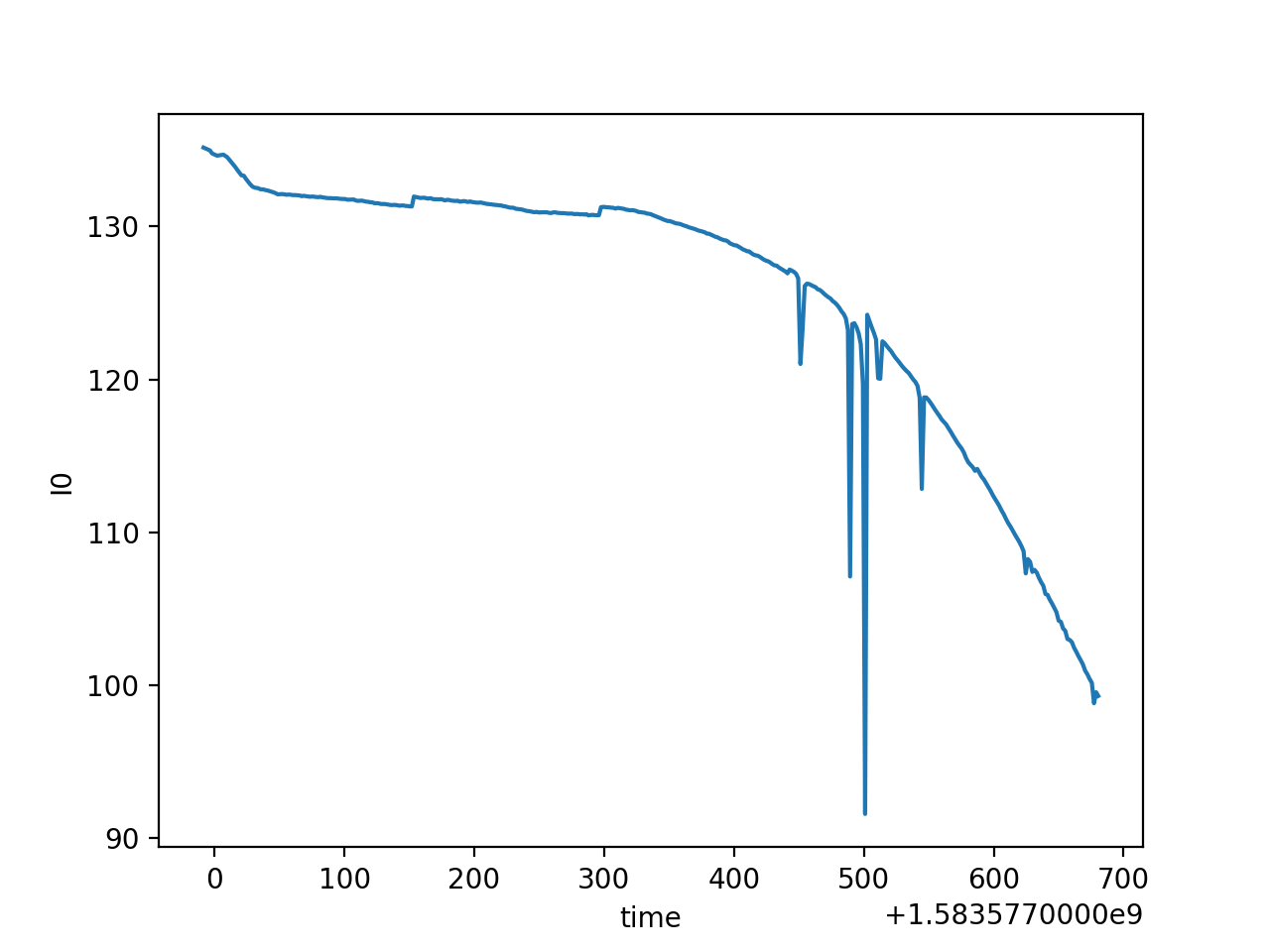
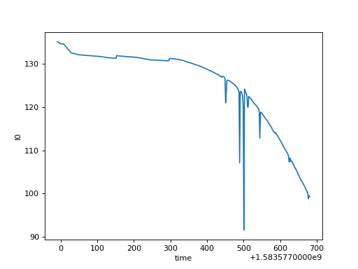
# The plot() method on xarray.DataArray
ds["I0"].plot()
(Source code, png, hires.png, pdf)
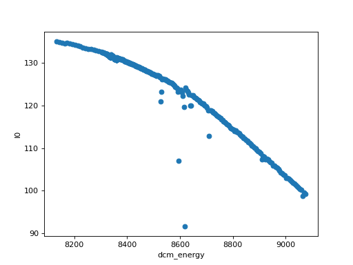
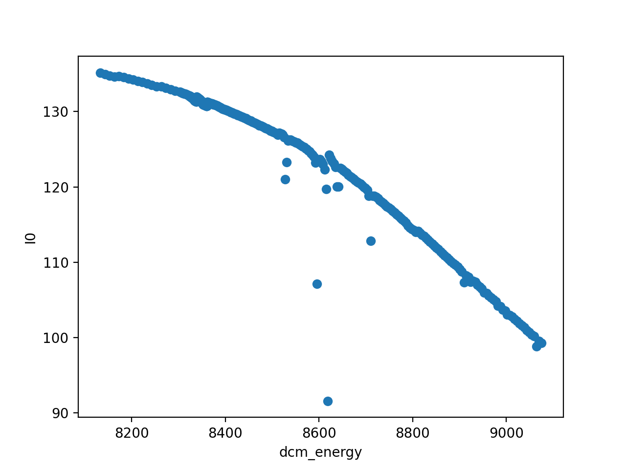
# The plot accessor on xarray.Dataset
ds.plot.scatter(x="dcm_energy", y="I0")
(Source code, png, hires.png, pdf)

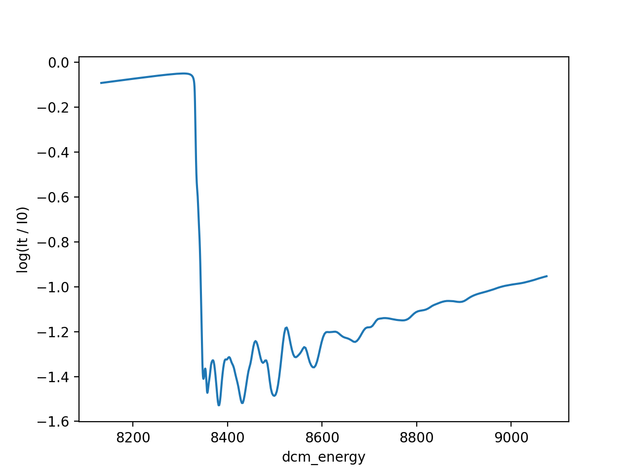
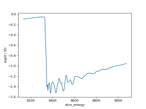
# Using matplotlib directly
import matplotlib.pyplot as plt
import numpy

plt.plot(ds["dcm_energy"], numpy.log(ds["It"] / ds["I0"]))
plt.xlabel("dcm_energy")
plt.ylabel("log(It / I0)")
(Source code, png, hires.png, pdf)
These xarray DataArray objects bundle a numpy (or numpy-like) array with
some additional metadata and coordinates. To access the underlying array
directly, use the data attribute.
In [13]: type(ds["I0"])
Out[13]: xarray.core.dataarray.DataArray

In [14]: type(ds["I0"].data)
Out[14]: numpy.ndarray
Looking again at this Run
In [15]: run
Out[15]:
BlueskyRun
  uid='4393404b-8986-4c75-9a64-d7f6949a9344'
  exit_status='success'
  2020-03-07 10:29:49.483 -- 2020-03-07 10:41:20.546
  Streams:
    * baseline
    * primary
we see it has a second stream, “baseline”. Reading that, we notice that columns it contains, its dimensions, and its coordinates are different from the ones in “primary”. That’s why it’s in a different stream. The “baseline” stream is a conventional name for snapshots taken at the very beginning and end of a procedure. We see a long list of instruments with two data points each—before and after.
In [16]: run.baseline.read()
Out[16]:
<xarray.Dataset>
Dimensions:                           (time: 2)
Coordinates:
  * time                              (time) float64 1.584e+09 1.584e+09
Data variables: (12/35)
    xafs_linxs                        (time) float64 -112.6 -112.6
    xafs_linxs_user_setpoint          (time) float64 -112.6 -112.6
    xafs_linxs_kill_cmd               (time) float64 1.0 1.0
    compton_shield_temperature        (time) float64 28.0 29.0
    xafs_wheel                        (time) float64 -2.655e+03 -2.655e+03
    xafs_wheel_user_setpoint          (time) float64 -2.655e+03 -2.655e+03
    ...                                ...
    xafs_liny                         (time) float64 102.9 102.9
    xafs_liny_user_setpoint           (time) float64 102.9 102.9
    xafs_liny_kill_cmd                (time) float64 1.0 1.0
    xafs_pitch                        (time) float64 1.735 1.735
    xafs_pitch_user_setpoint          (time) float64 1.735 1.735
    xafs_pitch_kill_cmd               (time) float64 1.0 1.0
Different Runs can have different streams, but “primary” and “baseline” are the two most common.
With that, we have accessed all the data from this run.
Handle large data
The example data we have been using so far has no large arrays in it. For this section we will download a second Catalog with one Run in it that contains image data. It’s 1 GB (uncompressed), which is large enough to exercise the tools involved. These same techniques scale to much larger datasets.
The large arrays require an extra reader, which we can get from the package
area-detector-handlers using pip on conda.
pip install area-detector-handlers
# or...
conda install -c nsls2forge area-detector-handlers
Scientificaly, this is Resonant Soft X-ray Scattering (RSoXS) data. (Details.)
In [17]: import databroker.tutorial_utils

In [18]: databroker.tutorial_utils.fetch_RSOXS_example()
Access the new Catalog and assign this Run to a variable.
In [19]: import databroker

In [20]: run = databroker.catalog['bluesky-tutorial-RSOXS']['777b44a']
In the previous example, we used run.primary.read() at this point. That
method reads all the data from the “primary” stream from storage into memory.
This can be inconvenient if:
The data is so large it does not all fit into memory (RAM) at once. Reading it would prompt a
MemoryError(best case) or cause Python to crash (worst case).You only need a subset of the data for your analysis. Reading all of it would waste time.
In these situations, we can summon up an xarray backed by placeholders (dask arrays). These act like normal numpy arrays in many respects, but internally they divide the data up intelligently into chunks. They only load the each chunk if and when it is actually needed for a computation.
In [21]: lazy_ds = run.primary.to_dask()
Comparing lazy_ds["Synced_waxs_image"].data to ds["I0"].data from the
previous section, we see that the “lazy” variant contains <dask.array ...>
and the original contains ordinary numpy array.
In [22]: ds["I0"].head().data  # array
Out[22]:
array([135.16644077, 134.97916279, 134.78557224, 134.63573771,
       134.70294218])

In [23]: lazy_ds["Synced_waxs_image"].data  # dask.array, a placeholder
Out[23]: dask.array<stack, shape=(128, 1, 1024, 1026), dtype=float64, chunksize=(1, 1, 1024, 1026), chunktype=numpy.ndarray>
As an example of what’s possible, we can subtract from this image series the mean of an image series taken while the shutter was closed (“dark” images).
In [24]: corrected = run.primary.to_dask()["Synced_waxs_image"] - run.dark.to_dask()["Synced_waxs_image"].mean("time")

In [25]: corrected
Out[25]:
<xarray.DataArray 'Synced_waxs_image' (time: 128, dim_3: 1, dim_4: 1024,
                                       dim_5: 1026)>
dask.array<sub, shape=(128, 1, 1024, 1026), dtype=float64, chunksize=(1, 1, 1024, 1026), chunktype=numpy.ndarray>
Coordinates:
  * time     (time) float64 1.574e+09 1.574e+09 ... 1.574e+09 1.574e+09
Dimensions without coordinates: dim_3, dim_4, dim_5

In [26]: middle_image = corrected[64, 0, :, :]  # Pull out a 2D slice.

In [27]: middle_image
Out[27]:
<xarray.DataArray 'Synced_waxs_image' (dim_4: 1024, dim_5: 1026)>
dask.array<getitem, shape=(1024, 1026), dtype=float64, chunksize=(1024, 1026), chunktype=numpy.ndarray>
Coordinates:
    time     float64 1.574e+09
Dimensions without coordinates: dim_4, dim_5
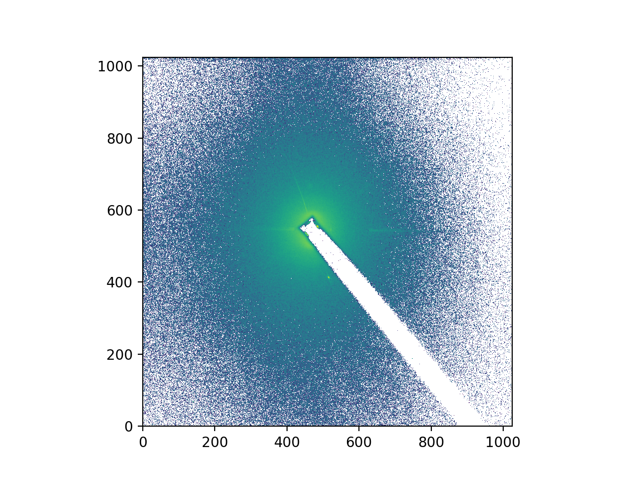
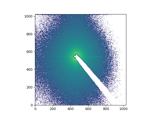
At this point, no data has yet been read. We are still working with placeholders, building up an expression of work to be done in the future. Finally, when we plot it or otherwise hand it off to code that will treat it as normal array, the data will be loaded and processed (in chunks) and finally give us a normal numpy array as a result. When only a sub-slice of the data is actually used—as is the case in this example—only the relevant chunk(s) will ever be loaded. This can save a lot of time and memory.
import matplotlib.pyplot as plt
from matplotlib.colors import LogNorm

# Plot a slice from the middle as an image with a log-scaled color transfer.
plt.imshow(middle_image, norm=LogNorm(), origin='lower')
(Source code, png, hires.png, pdf)
We can force that processing to happen explicitly by calling .compute().
In [28]: middle_image.compute()
Out[28]:
<xarray.DataArray 'Synced_waxs_image' (dim_4: 1024, dim_5: 1026)>
array([[ -9.33333333,  10.        , -12.33333333, ..., -19.        ,
        -22.        , -17.        ],
       [-30.66666667,   2.33333333,   0.66666667, ..., -20.33333333,
          2.66666667,  12.66666667],
       [ -0.33333333, -16.66666667, -23.66666667, ..., -26.33333333,
         15.66666667,  -7.66666667],
       ...,
       [ 10.        ,   0.33333333,  -9.66666667, ..., -22.66666667,
        -37.66666667, -25.33333333],
       [ -3.33333333,  -7.66666667,  -7.33333333, ...,   6.        ,
        -32.        , -12.        ],
       [ -5.        ,  -4.        ,  -2.33333333, ...,  -7.        ,
         16.33333333,  -6.        ]])
Coordinates:
    time     float64 1.574e+09
Dimensions without coordinates: dim_4, dim_5
Notice that we now see array in there instead of
<dask.array>. This is how we know that it’s a normal array in memory, not a
placeholder for future work.
For more, see the xarray documentation and the dask documentation. A good entry point is the example covering Dask Arrays.