4-circle diffractometer example
The IUCr provides a schematic of the 4-circle diffractometer (in horizontal geometry typical of a laboratory instrument).
E4CH geometry
At X-ray synchrotrons, the vertical geometry is more common due to the polarization of the X-rays.
Note: This example is available as a Jupyter notebook from the hklpy source code website: https://github.com/bluesky/hklpy/tree/main/examples
Load the hklpy package (named ``hkl``)
Since the hklpy package is a thin interface to the hkl library (compiled C++ code), we need to first load the gobject-introspection package (named ``gi``) and name our required code and version.
This is needed every time before the hkl package is first imported.
import gi
gi.require_version('Hkl', '5.0')
Setup the E4CV diffractometer in hklpy
In hkl E4CV geometry (https://people.debian.org/~picca/hkl/hkl.html#org7ef08ba):
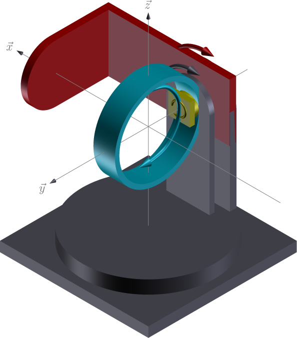
E4CV geometry
xrays incident on the \(\vec{x}\) direction (1, 0, 0)
axis |
moves |
rotation axis |
vector |
|---|---|---|---|
omega |
sample |
\(-\vec{y}\) |
|
chi |
sample |
\(\vec{x}\) |
|
phi |
sample |
\(-\vec{y}\) |
|
tth |
detector |
\(-\vec{y}\) |
|
Define this diffractometer
Create a python class that specifies the names of the real-space
positioners. We call it FourCircle here but that choice is
arbitrary. Pick any valid Python name not already in use.
The argument to the FourCircle class tells which hklpy base class
will be used. This sets the geometry. See the hklpy diffractometers
documentation
for a list of other choices.
In hklpy, the reciprocal-space axes are known as pseudo
positioners while the real-space axes are known as real positioners.
For the real positioners, it is possible to use different names than the
canonical names used internally by the hkl library. That is not
covered here.
note: The keyword argument kind="hinted" is an indication that this
signal may be plotted.
This demo uses simulated motors. To use EPICS motors, import that structure from ophyd:
from ophyd import EpicsMotor
Then, in the class, replace the real positioners with (substituting with the correct EPICS PV for each motor):
omega = Cpt(EpicsMotor, "pv_prefix:m41", kind="hinted")
chi = Cpt(EpicsMotor, "pv_prefix:m22", kind="hinted")
phi = Cpt(EpicsMotor, "pv_prefix:m35", kind="hinted")
tth = Cpt(EpicsMotor, "pv_prefix:m7", kind="hinted")
and, most important, remove the def __init__() method. It is
only needed to define an initial position for the simulators. Otherwise,
this will move these EPICS motors to zero.
from hkl.diffract import E4CV
from ophyd import PseudoSingle, SoftPositioner
from ophyd import Component as Cpt

class FourCircle(E4CV):
    """
    Our 4-circle.  Eulerian, vertical scattering orientation.
    """
    # the reciprocal axes are called: pseudo in hklpy
    h = Cpt(PseudoSingle, '', kind="hinted")
    k = Cpt(PseudoSingle, '', kind="hinted")
    l = Cpt(PseudoSingle, '', kind="hinted")

    # the motor axes are called: real in hklpy
    omega = Cpt(SoftPositioner, kind="hinted")
    chi = Cpt(SoftPositioner, kind="hinted")
    phi = Cpt(SoftPositioner, kind="hinted")
    tth = Cpt(SoftPositioner, kind="hinted")

    def __init__(self, *args, **kwargs):
        """Define an initial position for simulators."""
        super().__init__(*args, **kwargs)

        for p in self.real_positioners:
            p._set_position(0)  # give each a starting position
fourc = FourCircle("", name="fourc")
Add a sample with a crystal structure
from hkl.util import Lattice

# add the sample to the calculation engine
a0 = 5.431
fourc.calc.new_sample(
    "silicon",
    lattice=Lattice(a=a0, b=a0, c=a0, alpha=90, beta=90, gamma=90)
    )
HklSample(name='silicon', lattice=LatticeTuple(a=5.431, b=5.431, c=5.431, alpha=90.0, beta=90.0, gamma=90.0), ux=Parameter(name='None (internally: ux)', limits=(min=-180.0, max=180.0), value=0.0, fit=True, inverted=False, units='Degree'), uy=Parameter(name='None (internally: uy)', limits=(min=-180.0, max=180.0), value=0.0, fit=True, inverted=False, units='Degree'), uz=Parameter(name='None (internally: uz)', limits=(min=-180.0, max=180.0), value=0.0, fit=True, inverted=False, units='Degree'), U=array([[1., 0., 0.],
       [0., 1., 0.],
       [0., 0., 1.]]), UB=array([[ 1.15691131e+00, -7.08403864e-17, -7.08403864e-17],
       [ 0.00000000e+00,  1.15691131e+00, -7.08403864e-17],
       [ 0.00000000e+00,  0.00000000e+00,  1.15691131e+00]]), reflections=[])
Setup the UB orientation matrix using hklpy
Define the crystal’s orientation on the diffractometer using the 2-reflection method described by Busing & Levy, Acta Cryst 22 (1967) 457.
Choose the same wavelength X-rays for both reflections
fourc.calc.wavelength = 1.54 # Angstrom (8.0509 keV)
Find the first reflection and identify its Miller indices: (hkl)
r1 = fourc.calc.sample.add_reflection(
    4, 0, 0,
    position=fourc.calc.Position(
        tth=69.0966,
        omega=-145.451,
        chi=0,
        phi=0,
    )
)
Find the second reflection
r2 = fourc.calc.sample.add_reflection(
    0, 4, 0,
    position=fourc.calc.Position(
        tth=69.0966,
        omega=-145.451,
        chi=90,
        phi=0,
    )
)
Compute the UB orientation matrix
The compute_UB() method always returns 1. Ignore it.
fourc.calc.sample.compute_UB(r1, r2)
1
Report what we have setup
import pyRestTable

tbl = pyRestTable.Table()
tbl.labels = "term value".split()
tbl.addRow(("energy, keV", fourc.calc.energy))
tbl.addRow(("wavelength, angstrom", fourc.calc.wavelength))
tbl.addRow(("position", fourc.position))
tbl.addRow(("sample name", fourc.sample_name.get()))
tbl.addRow(("[U]", fourc.U.get()))
tbl.addRow(("[UB]", fourc.UB.get()))
tbl.addRow(("lattice", fourc.lattice.get()))
print(tbl)

print(f"sample\t{fourc.calc.sample}")
==================== ===================================================
term                 value
==================== ===================================================
energy, keV          8.050922077922078
wavelength, angstrom 1.54
position             FourCirclePseudoPos(h=-0.0, k=0.0, l=0.0)
sample name          silicon
[U]                  [[-1.22173048e-05 -1.22173048e-05 -1.00000000e+00]
                      [ 0.00000000e+00 -1.00000000e+00  1.22173048e-05]
                      [-1.00000000e+00  1.49262536e-10  1.22173048e-05]]
[UB]                 [[-1.41343380e-05 -1.41343380e-05 -1.15691131e+00]
                      [ 0.00000000e+00 -1.15691131e+00  1.41343380e-05]
                      [-1.15691131e+00  1.72683586e-10  1.41343380e-05]]
lattice              [ 5.431  5.431  5.431 90.    90.    90.   ]
==================== ===================================================

sample      HklSample(name='silicon', lattice=LatticeTuple(a=5.431, b=5.431, c=5.431, alpha=90.0, beta=90.0, gamma=90.0), ux=Parameter(name='None (internally: ux)', limits=(min=-180.0, max=180.0), value=-45.0, fit=True, inverted=False, units='Degree'), uy=Parameter(name='None (internally: uy)', limits=(min=-180.0, max=180.0), value=-89.99901005102187, fit=True, inverted=False, units='Degree'), uz=Parameter(name='None (internally: uz)', limits=(min=-180.0, max=180.0), value=135.00000000427607, fit=True, inverted=False, units='Degree'), U=array([[-1.22173048e-05, -1.22173048e-05, -1.00000000e+00],
       [ 0.00000000e+00, -1.00000000e+00,  1.22173048e-05],
       [-1.00000000e+00,  1.49262536e-10,  1.22173048e-05]]), UB=array([[-1.41343380e-05, -1.41343380e-05, -1.15691131e+00],
       [ 0.00000000e+00, -1.15691131e+00,  1.41343380e-05],
       [-1.15691131e+00,  1.72683586e-10,  1.41343380e-05]]), reflections=[(h=4.0, k=0.0, l=0.0), (h=0.0, k=4.0, l=0.0)], reflection_measured_angles=array([[0.        , 1.57079633],
       [1.57079633, 0.        ]]), reflection_theoretical_angles=array([[0.        , 1.57079633],
       [1.57079633, 0.        ]]))
Check the orientation matrix
Perform checks with forward (hkl to angle) and inverse (angle to hkl) computations to verify the diffractometer will move to the same positions where the reflections were identified.
Constrain the motors to limited ranges
allow for slight roundoff errors
keep
tthin the positive rangekeep
omegain the negative rangekeep
phifixed at zero
fourc.calc["tth"].limits = (-0.001, 180)
fourc.calc["omega"].limits = (-180, 0.001)

fourc.phi.move(0)
fourc.engine.mode = "constant_phi"
(400) reflection test
Check the
inverse(angles -> (hkl)) computation.Check the
forward((hkl) -> angles) computation.
Check the inverse calculation: (400)
To calculate the (hkl) corresponding to a given set of motor angles,
call fourc.inverse((h, k, l)). Note the second set of parentheses
needed by this function.
The values are specified, without names, in the order specified by
fourc.calc.physical_axis_names.
print("axis names:", fourc.calc.physical_axis_names)
axis names: ['omega', 'chi', 'phi', 'tth']
Now, proceed with the inverse calculation.
sol = fourc.inverse((-145.451, 0, 0, 69.0966))
print("(4 0 0) ?", f"{sol.h:.2f}", f"{sol.k:.2f}", f"{sol.l:.2f}")
(4 0 0) ? 4.00 0.00 0.00
Check the forward calculation: (400)
Compute the angles necessary to position the diffractometer for the given reflection.
Note that for the forward computation, more than one set of angles may
be used to reach the same crystal reflection. This test will report the
default selection. The default selection (which may be changed
through methods described in the hkl.calc module) is the first
solution.
function |
returns |
|---|---|
|
The default solution |
|
List of all allowed solutions. |
sol = fourc.forward((4, 0, 0))
print(
    "(400) :",
    f"tth={sol.tth:.4f}",
    f"omega={sol.omega:.4f}",
    f"chi={sol.chi:.4f}",
    f"phi={sol.phi:.4f}"
    )
(400) : tth=69.0985 omega=-145.4500 chi=0.0000 phi=0.0000
(040) reflection test
Repeat the inverse and forward calculations for the second
orientation reflection.
Check the inverse calculation: (040)
sol = fourc.inverse((-145.451, 90, 0, 69.0966))
print("(0 4 0) ?", f"{sol.h:.2f}", f"{sol.k:.2f}", f"{sol.l:.2f}")
(0 4 0) ? 0.00 4.00 0.00
Check the forward calculation: (040)
sol = fourc.forward((0, 4, 0))
print(
    "(040) :",
    f"tth={sol.tth:.4f}",
    f"omega={sol.omega:.4f}",
    f"chi={sol.chi:.4f}",
    f"phi={sol.phi:.4f}"
    )
(040) : tth=69.0985 omega=-145.4500 chi=90.0000 phi=0.0000
(440) reflection: angles
sol = fourc.forward((4, 4, 0))
print(
    "(440) :",
    f"tth={sol.tth:.4f}",
    f"omega={sol.omega:.4f}",
    f"chi={sol.chi:.4f}",
    f"phi={sol.phi:.4f}"
    )
(440) : tth=106.6471 omega=-126.6755 chi=45.0000 phi=0.0000
Scan in reciprocal space using Bluesky
To scan with Bluesky, we need more setup.
%matplotlib inline

from bluesky import RunEngine
from bluesky import SupplementalData
from bluesky.callbacks.best_effort import BestEffortCallback
import bluesky.plans as bp
import bluesky.plan_stubs as bps
import databroker
import matplotlib.pyplot as plt

plt.ion()

bec = BestEffortCallback()
db = databroker.temp().v1
sd = SupplementalData()

RE = RunEngine({})
RE.md = {}
RE.preprocessors.append(sd)
RE.subscribe(db.insert)
RE.subscribe(bec)
1
(h00) scan near (400)
RE(bp.scan([], fourc.h, 3.9, 4.1, 5))
Transient Scan ID: 1     Time: 2020-12-09 12:02:58
Persistent Unique Scan ID: '26088e62-fd00-40ec-bfd3-fccf3a4d320d'
New stream: 'primary'
+-----------+------------+------------+
|   seq_num |       time |    fourc_h |
+-----------+------------+------------+
|         1 | 12:02:58.3 |      3.900 |
|         2 | 12:02:58.3 |      3.950 |
|         3 | 12:02:58.3 |      4.000 |
|         4 | 12:02:58.3 |      4.050 |
|         5 | 12:02:58.3 |      4.100 |
+-----------+------------+------------+
generator scan ['26088e62'] (scan num: 1)
('26088e62-fd00-40ec-bfd3-fccf3a4d320d',)
chi scan from (400) to (040)
RE(bp.scan([fourc.chi, fourc.h, fourc.k, fourc.l], fourc.chi, 0, 90, 10))
Transient Scan ID: 2     Time: 2020-12-09 12:02:58
Persistent Unique Scan ID: '8072de45-4a80-4e47-9df9-151623ace6ff'
New stream: 'primary'
+-----------+------------+------------+------------+------------+------------+
|   seq_num |       time |  fourc_chi |    fourc_k |    fourc_l |    fourc_h |
+-----------+------------+------------+------------+------------+------------+
|         1 | 12:02:58.7 |      0.000 |      0.000 |      0.000 |      4.100 |
|         2 | 12:02:58.9 |     10.000 |      0.712 |     -0.000 |      4.038 |
|         3 | 12:02:59.2 |     20.000 |      1.402 |     -0.000 |      3.853 |
|         4 | 12:02:59.4 |     30.000 |      2.050 |     -0.000 |      3.551 |
|         5 | 12:02:59.7 |     40.000 |      2.635 |     -0.000 |      3.141 |
|         6 | 12:02:59.9 |     50.000 |      3.141 |     -0.000 |      2.635 |
|         7 | 12:03:00.1 |     60.000 |      3.551 |     -0.000 |      2.050 |
|         8 | 12:03:00.3 |     70.000 |      3.853 |     -0.000 |      1.402 |
|         9 | 12:03:00.6 |     80.000 |      4.038 |     -0.000 |      0.712 |
|        10 | 12:03:00.8 |     90.000 |      4.100 |      0.000 |      0.000 |
+-----------+------------+------------+------------+------------+------------+
generator scan ['8072de45'] (scan num: 2)
('8072de45-4a80-4e47-9df9-151623ace6ff',)

(0k0) scan near (040)
RE(bp.scan([], fourc.k, 3.9, 4.1, 5))
Transient Scan ID: 3     Time: 2020-12-09 12:03:01
Persistent Unique Scan ID: 'aa3ef21b-80d2-472b-a459-d5bd30cae54a'
New stream: 'primary'
+-----------+------------+------------+
|   seq_num |       time |    fourc_k |
+-----------+------------+------------+
|         1 | 12:03:01.9 |      3.900 |
|         2 | 12:03:01.9 |      3.950 |
|         3 | 12:03:01.9 |      4.000 |
|         4 | 12:03:01.9 |      4.050 |
|         5 | 12:03:01.9 |      4.100 |
+-----------+------------+------------+
generator scan ['aa3ef21b'] (scan num: 3)
('aa3ef21b-80d2-472b-a459-d5bd30cae54a',)
(hk0) scan near (440)
RE(bp.scan([], fourc.h, 3.9, 4.1, fourc.k, 3.9, 4.1, 5))
Transient Scan ID: 4     Time: 2020-12-09 12:03:02
Persistent Unique Scan ID: '36abd81c-c313-4035-acde-67782c2908d1'
New stream: 'primary'
+-----------+------------+------------+------------+------------+-------------+------------+------------+------------+
|   seq_num |       time |    fourc_h |    fourc_k |    fourc_l | fourc_omega |  fourc_chi |  fourc_phi |  fourc_tth |
+-----------+------------+------------+------------+------------+-------------+------------+------------+------------+
|         1 | 12:03:02.4 |      3.900 |      3.900 |      0.000 |    -128.558 |     45.000 |      0.000 |    102.883 |
|         2 | 12:03:03.0 |      3.950 |      3.950 |     -0.000 |    -127.627 |     45.000 |      0.000 |    104.745 |
|         3 | 12:03:03.7 |      4.000 |      4.000 |     -0.000 |    -126.675 |     45.000 |      0.000 |    106.647 |
|         4 | 12:03:04.3 |      4.050 |      4.050 |     -0.000 |    -125.703 |     45.000 |      0.000 |    108.593 |
|         5 | 12:03:05.0 |      4.100 |      4.100 |      0.000 |    -124.706 |     45.000 |      0.000 |    110.585 |
+-----------+------------+------------+------------+------------+-------------+------------+------------+------------+
generator scan ['36abd81c'] (scan num: 4)
('36abd81c-c313-4035-acde-67782c2908d1',)
