Hello Python and Jupyter
Contents
Hello Python and Jupyter#
In this notebook you will:
Learn how to use a Jupyter notebook such as this one
Get a very quick tour of Python syntax and scientific libraries
Learn some IPython features that we will use in later tutorials
What is this?#
This is Jupyter notebook running in a personal “container” just for you, stocked with example data, demos, and tutorials that you can run and modify. All of the software you’ll need is already installed and ready to use.
Run some Python code!#
To run the code below:
Click on the cell to select it.
Press
SHIFT+ENTERon your keyboard or press the button in the toolbar above (in the toolbar above!).
1 + 1
2
Notice that you can edit a cell and re-run it.
The notebook document mixes executable code and narrative content. It supports text, links, embedded videos, and even typeset math: \(\int_{-\infty}^\infty x\, d x = \frac{x^2}{2}\)
Whirlwind Tour of Python Syntax#
Lists#
stuff = [4, 'a', 8.3, True]
stuff[0] # the first element
4
stuff[-1] # the last element
True
Dictionaries (Mappings)#
d = {'a': 1, 'b': 2}
d
{'a': 1, 'b': 2}
d['b']
2
d['c'] = 3
d
{'a': 1, 'b': 2, 'c': 3}
TIP: For large or nested dictionaries, it is more convient to use list(). Often custom python objects can be interrogated in the same manner.
list(d)
['a', 'b', 'c']
Functions#
def f(a, b):
    return a + b
In IPython f? or ?f display information about f, such as its arguments.
f?
If the function includes inline documentation (a “doc string”) then ? displays that as well.
def f(a, b):
    "Add a and b."
    return a + b
f?
f??
Arguments can have default values.
def f(a, b, c=1):
    return (a + b) * c
f(1, 2)
3
f(1, 2, 3)
9
Any argument can be passed by keyword. This is slower to type but clearer to read later.
f(a=1, b=2, c=3)
9
If using keywords, you don’t have to remember the argument order.
f(c=3, a=1, b=2)
9
Fast numerical computation using numpy#
For numerical computing, a numpy array is more useful and performant than a plain list.
import numpy as np

a = np.array([1, 2, 3, 4])
a
array([1, 2, 3, 4])
np.mean(a)
2.5
np.sin(a)
array([ 0.84147098, 0.90929743, 0.14112001, -0.7568025 ])
We’ll use the IPython %%timeit magic to measure the speed difference between built-in Python lists and numpy arrays.
%%timeit

big = list(range(10000))  # setup line, not timed
sum(big)  # timed
183 µs ± 58.8 ns per loop (mean ± std. dev. of 7 runs, 10,000 loops each)
%%timeit

big = np.arange(10000)  # setup line, not timed
np.sum(big)  # timed
11.5 µs ± 8.35 ns per loop (mean ± std. dev. of 7 runs, 100,000 loops each)
If a single loops is desired for a longer computation, use %time on the desired line.
big = np.arange(10000)  # setup line, not timed
%time np.sum(big)  # timed
CPU times: user 41 µs, sys: 0 ns, total: 41 µs
Wall time: 39.3 µs
49995000
Plotting using matplotlib#
In an interactive setting, this will show a canvas that we can pan and zoom. (Keep reading for what we can do in a non-interactive setting, such as the static web page version of this tutorial.)
# We just have to do this line once, before we do any plotting.
%matplotlib widget
import matplotlib.pyplot as plt

plt.figure()
<Figure size 640x480 with 0 Axes>
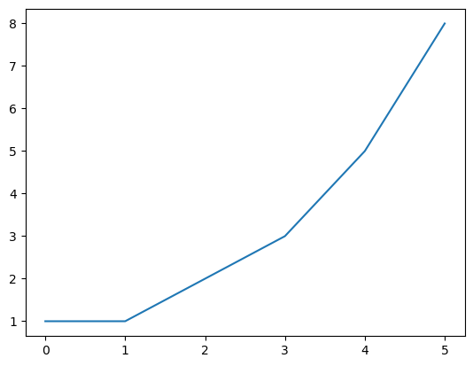
We can plot some data like so. In an interactive setting, this will update the canvas above.
plt.plot([1, 1, 2, 3, 5, 8])
[<matplotlib.lines.Line2D at 0x7f8fa4914790>]
And we can show a noninteractive snapshot of the state of the figure at this point by display the figure itself.
plt.gcf()
Displaying plt.gcf() (or any Figure) shows a non-interactive snapshot of a figure. Displaying plt.gcf().canvas or any Canvas gives us another interactive, live-updating view of the figure.
Interrupting the IPython Kernel#
Run this cell, and then click the square ‘stop’ button in the notebook toolbar to interrupt the infinite loop.
(This is equivalent to Ctrl+C in a terminal.)
# This runs forever -- hit the square 'stop' button in Jupyter to interrupt
# The following is "commented out". Un-comment the lines below to run them.
# while True:
#     continue
“Magics”#
The code entered here is interpreted by IPython, which extends Python by adding some conveniences that help you make the most out of using Python interactively. It was originally created by a physicist, Fernando Perez.
“Magics” are special IPython syntax. They are not part of the Python language, and they should not be used in scripts or libraries; they are meant for interactive use.
The %run magic executes a Python script.
%run scripts/hello_world.py
hello world
When the script completes, any variables defined in that script will be dumepd into our namespace. For example (as we will see below), this script happens to define a variable named message. Now that we have %run the script, message is in our namespace.
message
'hello world'
This behavior can be confusing, in the sense that the reader has to do some digging to figure out where message was defined and what it is, but it has its uses. Throughout this tutorial, we will use the %run magic as a shorthand for running boilerplate configuration code and defining variables representing hardware.
The %load magic copies the contents of a file into a cell but does not run it.
%load scripts/hello_world.py
Execute the cell a second time to actually run the code. Throughout this tutorial, we use the %load magic to load solutions to exercises.
System Shell Access#
Any input line beginning with a ! character is passed verbatim (minus the !, of course) to the underlying operating system.
!ls
'Access Saved Data.ipynb'	        LICENSE
'Access Saved Data Via the Web.ipynb'   Ophyd
'Adaptive RL Sampling'		        README.md
 archive			        scripts
 binder				       'Single PVs.ipynb'
 bluesky-tutorial-utils		        solutions
 _build				        static
 _config.yml			        STATUS.md
 CONTRIBUTING.md		        supervisor
'Hello Bluesky.ipynb'		        _toc.yml
'Hello Python and Jupyter.ipynb'        Welcome.md
 INSTALLATION.md		       'X-ray Absorption Fine Structure'
 launch.sh