Optimizing KB Mirrors with Bayesian Optimization#
In this tutorial, you will learn how to use Blop to optimize a Kirkpatrick-Baez (KB) mirror system. By the end, you will understand:
How degrees of freedom (DOFs) represent the parameters you can adjust in an experiment
How objectives define what you’re trying to optimize
How tracking metrics let you monitor values without optimizing them
How to write an evaluation function that extracts results from experimental data
How the Agent coordinates the optimization loop
How to check optimization health mid-run and continue
We’ll work with a simulated KB mirror beamline, but the concepts apply directly to real experimental setups.
What are KB Mirrors?#
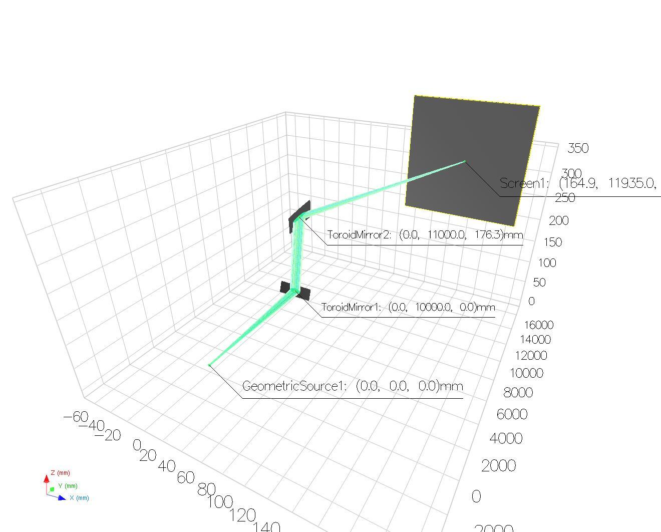
KB mirror systems use two curved mirrors to focus X-ray beams. Each mirror has adjustable curvature—getting both just right produces a tight, intense focal spot. We’ll frame this as a single-objective optimization problem: minimize the beam’s FWHM (full width at half maximum) on the detector, subject to a minimum intensity constraint.
The image below shows our simulated setup: a beam from a geometric source propagates through a pair of toroidal mirrors that focus it onto a screen.
Setting Up the Environment#
Before we can optimize, we need to set up the data infrastructure. Blop uses Bluesky to run experiments and Tiled to store and retrieve data.
import logging
import warnings
from pathlib import PurePath
import matplotlib.pyplot as plt
import numpy as np
from ax.api.protocols import IMetric
from bluesky.run_engine import RunEngine
from bluesky_tiled_plugins import TiledWriter
from ophyd_async.core import StaticPathProvider, UUIDFilenameProvider
from tiled.client import from_uri # type: ignore[import-untyped]
from tiled.client.container import Container
from tiled.server import SimpleTiledServer
from blop.ax import Agent, Objective, RangeDOF
from blop.ax.objective import OutcomeConstraint
from blop.protocols import EvaluationFunction
# Import simulation devices (requires: pip install -e sim/)
from blop_sim.backends.xrt import XRTBackend
from blop_sim.devices import DetectorDevice
from blop_sim.devices.xrt import KBMirror
# Suppress noisy logs from httpx and dependency deprecation warnings
logging.getLogger("httpx").setLevel(logging.WARNING)
warnings.filterwarnings("ignore", category=FutureWarning)
# Enable interactive plotting
plt.ion()
DETECTOR_STORAGE = "/tmp/blop/sim"
[INFO 06-08 19:45:16] ax.storage.sqa_store.with_db_settings_base: Ax SQL storage initialized with SQLAlchemy 2.0.50
/home/runner/work/blop/blop/.pixi/envs/docs/lib/python3.13/site-packages/xrt/backends/raycing/sources/sybase.py:78: SyntaxWarning: invalid escape sequence '\s'
:math:`\beta_i = \frac{\sigma_i^{2}}{\epsilon_i}`, with
Next, we create a local Tiled server. The TiledWriter callback will save experimental data to this server, and our evaluation function will read from it.
tiled_server = SimpleTiledServer(readable_storage=[DETECTOR_STORAGE])
tiled_client = from_uri(tiled_server.uri)
tiled_writer = TiledWriter(tiled_client)
RE = RunEngine({})
RE.subscribe(tiled_writer)
Tiled version 0.2.11
0
Defining Degrees of Freedom#
Degrees of freedom (DOFs) are the parameters the optimizer can adjust. In our KB system, we control the curvature radius of each mirror. Let’s define the search space:
# Define search ranges for each mirror's curvature radius
# The optimal values (~38000 and ~21000) are intentionally placed
# away from the center to make the optimization more realistic
VERTICAL_BOUNDS = (25000, 45000) # Optimal ~38000 is in upper portion
HORIZONTAL_BOUNDS = (15000, 35000) # Optimal ~21000 is in lower portion
Now we create the simulation backend and individual devices. Each RangeDOF wraps an actuator (something we can move) with bounds that constrain the search space:
# Create XRT simulation backend
backend = XRTBackend()
# Create individual KB mirror devices
kbv = KBMirror(backend, mirror_index=0, initial_radius=38000, name="kbv")
kbh = KBMirror(backend, mirror_index=1, initial_radius=21000, name="kbh")
# Create detector device
det = DetectorDevice(backend, StaticPathProvider(UUIDFilenameProvider(), PurePath(DETECTOR_STORAGE)), name="det")
# Define DOFs using mirror radius signals
dofs = [
RangeDOF(actuator=kbv.radius, bounds=VERTICAL_BOUNDS, parameter_type="float"),
RangeDOF(actuator=kbh.radius, bounds=HORIZONTAL_BOUNDS, parameter_type="float"),
]
The actuator is the device that physically changes the parameter. The bounds tell the optimizer what range of values to explore. Think of DOFs as the “knobs” the optimizer can turn.
Defining the Objective and Constraints#
For beam focusing, we use a single objective: minimize the beam FWHM (full width at half maximum). This is more sample-efficient than multi-objective optimization because the optimizer only needs to model one response surface.
We also track intensity as a metric without optimizing it directly. An OutcomeConstraint ensures the optimizer avoids configurations where the beam misses the detector entirely:
# Single objective: minimize the geometric-mean FWHM
objectives = [
Objective(name="fwhm", minimize=True),
]
# Track intensity without optimizing it
intensity_metric = IMetric(name="intensity")
# Soft constraint: reject configurations where most rays miss the screen
outcome_constraints = [
OutcomeConstraint(constraint="i >= 10000", i=intensity_metric),
]
Using a single objective with an outcome constraint gives us the best of both worlds: focused optimization on spot size, with a safety net ensuring we don’t “optimize” toward configurations where the beam is simply lost.
Writing an Evaluation Function#
The evaluation function is the bridge between raw experimental data and the optimizer. After each measurement, the optimizer needs to know how well that configuration performed. Our evaluation function:
Receives a run UID and the suggestions that were tested
Reads the beam images from Tiled
Computes FWHM from the marginal beam profiles
Returns outcome values for each suggestion
We compute FWHM using marginal profiles — projecting the 2D image onto each axis by summing, then finding where the 1D profile crosses half its peak value. This approach is robust to noise and dead pixels (they get averaged out in the projection) and doesn’t require curve fitting.
class DetectorEvaluation(EvaluationFunction):
def __init__(self, tiled_client: Container):
self.tiled_client = tiled_client
def _fwhm_from_profile(self, profile: np.ndarray) -> float:
"""Compute FWHM from a 1D marginal profile.
Finds the half-maximum crossing points with sub-pixel interpolation.
Returns a large value if the beam is too dim or fills the entire detector.
"""
peak = profile.max()
if peak == 0:
return float(len(profile)) # No signal — return detector width as penalty
half_max = peak / 2.0
above = profile >= half_max
if not above.any():
return float(len(profile))
indices = np.where(above)[0]
left_idx = indices[0]
right_idx = indices[-1]
# Sub-pixel interpolation at left crossing
if left_idx > 0:
left = left_idx - 1 + (half_max - profile[left_idx - 1]) / (profile[left_idx] - profile[left_idx - 1])
else:
left = 0.0
# Sub-pixel interpolation at right crossing
if right_idx < len(profile) - 1:
right = right_idx + (half_max - profile[right_idx]) / (profile[right_idx + 1] - profile[right_idx])
else:
right = float(len(profile) - 1)
return right - left
def _compute_stats(self, image: np.ndarray) -> tuple[float, float]:
"""Compute FWHM and integrated intensity from a beam image.
Returns
-------
fwhm : float
Geometric mean of the horizontal and vertical FWHM (in pixels).
intensity : float
Total integrated intensity (sum of all pixel values).
"""
gray = image.squeeze().astype(np.float64)
if gray.ndim == 3:
gray = gray.mean(axis=-1)
# Integrated intensity (total flux on detector)
intensity = gray.sum()
if intensity == 0:
return 400.0, 0.0 # No beam — return max FWHM penalty
# Marginal profiles: project onto each axis
x_profile = gray.sum(axis=0) # sum along Y rows -> X profile
y_profile = gray.sum(axis=1) # sum along X cols -> Y profile
fwhm_x = self._fwhm_from_profile(x_profile)
fwhm_y = self._fwhm_from_profile(y_profile)
# Geometric mean FWHM — targets a small, round spot
fwhm = np.sqrt(fwhm_x * fwhm_y)
return float(fwhm), float(intensity)
def __call__(self, uid: str, suggestions: list[dict]) -> list[dict]:
outcomes = []
run = self.tiled_client[uid]
# Read beam images from detector
images = run["primary/det_image"].read()
# Suggestion IDs stored in start document metadata
suggestion_ids = [suggestion["_id"] for suggestion in run.metadata["start"]["blop_suggestions"]]
# Compute statistics from each image
for idx, sid in enumerate(suggestion_ids):
image = images[idx]
fwhm, intensity = self._compute_stats(image)
outcome = {
"_id": sid,
"fwhm": fwhm,
"intensity": intensity,
}
outcomes.append(outcome)
return outcomes
Note how we:
Project the 2D image onto each axis to get 1D profiles
Find the FWHM of each profile using half-maximum crossings
Combine them into a single geometric-mean FWHM metric
Track integrated intensity for the outcome constraint
Link each outcome back to its suggestion via the
_idfield
Creating and Running the Agent#
The Agent brings everything together. It:
Uses DOFs to know what parameters to adjust
Uses objectives to know what to optimize
Calls the evaluation function to assess each configuration
Builds a surrogate model to predict outcomes across the parameter space
Suggests the next configurations to try
agent = Agent(
sensors=[det],
dofs=dofs,
objectives=objectives,
evaluation_function=DetectorEvaluation(tiled_client),
outcome_constraints=outcome_constraints,
name="xrt-blop-demo",
description="A demo of the Blop agent with XRT simulated beamline",
experiment_type="demo",
)
# Register intensity as a tracking metric (monitored but not optimized)
agent.ax_client.configure_metrics([intensity_metric])
The sensors list contains any devices that produce data during acquisition. The outcome_constraints tell the optimizer to prefer configurations satisfying the intensity constraint. The configure_metrics call registers intensity as a tracking metric so it appears in analyses and summaries.
Running the Optimization#
Let’s start the optimization. We’ll begin with a batch of 10 points to build an initial model of the parameter space—this includes a center-of-space sample plus quasi-random exploration points.
# Run 1 iteration with a batch of 10 points for initial exploration
RE(agent.optimize(1, n_points=10))
╭───────────────────────────────────────────────── Optimization ──────────────────────────────────────────────────╮ │ Optimizer AxOptimizer │ │ Actuators kbv-radius, kbh-radius │ │ Sensors det │ │ Iterations 1 Points/iter 10 │ │ Run UID 317309ab-119e-4d73-8d1f-1e0503942e10 │ ╰─────────────────────────────────────────────────────────────────────────────────────────────────────────────────╯
[INFO 06-08 19:45:22] ax.api.client: GenerationStrategy(name='Center+Sobol+MBM:fast', nodes=[CenterGenerationNode(next_node_name='Sobol', use_existing_trials_for_initialization=True), GenerationNode(name='Sobol', generator_specs=[GeneratorSpec(generator_enum=Sobol, generator_key_override=None)], transition_criteria=[MinTrials(transition_to='MBM'), MinTrials(transition_to='MBM')], suggested_experiment_status=ExperimentStatus.INITIALIZATION, pausing_criteria=[MaxTrialsAwaitingData(threshold=5)]), GenerationNode(name='MBM', generator_specs=[GeneratorSpec(generator_enum=BoTorch, generator_key_override=None)], transition_criteria=None, suggested_experiment_status=ExperimentStatus.OPTIMIZATION, pausing_criteria=None)]) chosen based on user input and problem structure.
[INFO 06-08 19:45:22] ax.api.client: Generated new trial 0 with parameters {'kbv-radius': 35000.0, 'kbh-radius': 25000.0} using GenerationNode CenterOfSearchSpace.
[INFO 06-08 19:45:22] ax.api.client: Generated new trial 1 with parameters {'kbv-radius': 35549.819469, 'kbh-radius': 26942.349672} using GenerationNode Sobol.
[INFO 06-08 19:45:22] ax.api.client: Generated new trial 2 with parameters {'kbv-radius': 33956.873361, 'kbh-radius': 17417.120002} using GenerationNode Sobol.
[INFO 06-08 19:45:22] ax.api.client: Generated new trial 3 with parameters {'kbv-radius': 29461.896531, 'kbh-radius': 30788.192991} using GenerationNode Sobol.
[INFO 06-08 19:45:22] ax.api.client: Generated new trial 4 with parameters {'kbv-radius': 40991.509464, 'kbh-radius': 20955.233276} using GenerationNode Sobol.
[INFO 06-08 19:45:22] ax.api.client: Generated new trial 5 with parameters {'kbv-radius': 44443.756975, 'kbh-radius': 33852.021191} using GenerationNode Sobol.
[INFO 06-08 19:45:22] ax.api.client: Generated new trial 6 with parameters {'kbv-radius': 26039.135437, 'kbh-radius': 24326.961488} using GenerationNode Sobol.
[INFO 06-08 19:45:22] ax.api.client: Generated new trial 7 with parameters {'kbv-radius': 30543.315485, 'kbh-radius': 27774.731424} using GenerationNode Sobol.
[INFO 06-08 19:45:22] ax.api.client: Generated new trial 8 with parameters {'kbv-radius': 39011.252392, 'kbh-radius': 17942.16942} using GenerationNode Sobol.
[INFO 06-08 19:45:22] ax.api.client: Generated new trial 9 with parameters {'kbv-radius': 37963.716146, 'kbh-radius': 31428.349894} using GenerationNode Sobol.
[INFO 06-08 19:45:23] ax.api.client: Trial 2 marked COMPLETED.
[INFO 06-08 19:45:23] ax.api.client: Trial 0 marked COMPLETED.
[INFO 06-08 19:45:23] ax.api.client: Trial 1 marked COMPLETED.
[INFO 06-08 19:45:23] ax.api.client: Trial 7 marked COMPLETED.
[INFO 06-08 19:45:23] ax.api.client: Trial 6 marked COMPLETED.
[INFO 06-08 19:45:23] ax.api.client: Trial 3 marked COMPLETED.
[INFO 06-08 19:45:23] ax.api.client: Trial 9 marked COMPLETED.
[INFO 06-08 19:45:23] ax.api.client: Trial 5 marked COMPLETED.
[INFO 06-08 19:45:23] ax.api.client: Trial 4 marked COMPLETED.
[INFO 06-08 19:45:23] ax.api.client: Trial 8 marked COMPLETED.
────────────────────────────────────────── Iteration 1 / 1 (10 points) ───────────────────────────────────────────
Acquire UID ee1a4c40-8705-42cc-b301-9dce485bc94c
┏━━━━━━━┳━━━━━━━━━━━━━━━┳━━━━━━━━━━━━┳━━━━━━━━━━━━┳━━━━━━━━━┳━━━━━━━━━━━┓ ┃ Event ┃ Suggestion ID ┃ kbh-radius ┃ kbv-radius ┃ fwhm ┃ intensity ┃ ┡━━━━━━━╇━━━━━━━━━━━━━━━╇━━━━━━━━━━━━╇━━━━━━━━━━━━╇━━━━━━━━━╇━━━━━━━━━━━┩ │ 0 │ 0 │ 25000 │ 35000 │ 141.087 │ 46976 │ │ 1 │ 1 │ 26942.3 │ 35549.8 │ 153.035 │ 41996 │ │ 2 │ 2 │ 17417.1 │ 33956.9 │ 165.425 │ 45930 │ │ 3 │ 3 │ 30788.2 │ 29461.9 │ 323.678 │ 27246 │ │ 4 │ 4 │ 20955.2 │ 40991.5 │ 37.7576 │ 50000 │ │ 5 │ 5 │ 33852 │ 44443.8 │ 225.866 │ 29537 │ │ 6 │ 6 │ 24327 │ 26039.1 │ 248.778 │ 27873 │ │ 7 │ 7 │ 27774.7 │ 30543.3 │ 278.875 │ 34642 │ │ 8 │ 8 │ 17942.2 │ 39011.3 │ 84.6849 │ 48080 │ │ 9 │ 9 │ 31428.3 │ 37963.7 │ 95.6693 │ 32922 │ └───────┴───────────────┴────────────┴────────────┴─────────┴───────────┘
fwhm min: 37.7576 max: 323.678 mean: 175.486 intensity min: 27246 max: 50000 mean: 38520.2 (10 pts sampled)
Summary Statistics ┏━━━━━━━━━━━━┳━━━━━━━━━┳━━━━━━━━━┳━━━━━━━━━┳━━━━━━━━━┳━━━━━━━━━┳━━━━━━━┓ ┃ Name ┃ Type ┃ Min ┃ Max ┃ Mean ┃ Std ┃ Count ┃ ┡━━━━━━━━━━━━╇━━━━━━━━━╇━━━━━━━━━╇━━━━━━━━━╇━━━━━━━━━╇━━━━━━━━━╇━━━━━━━┩ │ kbh-radius │ param │ 17417.1 │ 33852 │ 25642.7 │ 5623.88 │ 10 │ │ kbv-radius │ param │ 26039.1 │ 44443.8 │ 35296.1 │ 5590.66 │ 10 │ │ fwhm │ outcome │ 37.7576 │ 323.678 │ 175.486 │ 91.8532 │ 10 │ │ intensity │ outcome │ 27246 │ 50000 │ 38520.2 │ 9001.3 │ 10 │ └────────────┴─────────┴─────────┴─────────┴─────────┴─────────┴───────┘
────────────────────────────────────────────── Optimization Complete ──────────────────────────────────────────────
('317309ab-119e-4d73-8d1f-1e0503942e10',
'ee1a4c40-8705-42cc-b301-9dce485bc94c')
Continuing the Optimization#
The optimization state is preserved, so we can simply run more iterations:
# Run remaining 10 iterations
RE(agent.optimize(10))
╭───────────────────────────────────────────────── Optimization ──────────────────────────────────────────────────╮ │ Optimizer AxOptimizer │ │ Actuators kbv-radius, kbh-radius │ │ Sensors det │ │ Iterations 10 more (1 completed, 11 total) │ │ Run UID 81608068-3985-4f56-a529-40fa45a16937 │ ╰─────────────────────────────────────────────────────────────────────────────────────────────────────────────────╯
[INFO 06-08 19:45:24] ax.api.client: Generated new trial 10 with parameters {'kbv-radius': 40220.468065, 'kbh-radius': 24362.793988} using GenerationNode MBM.
[INFO 06-08 19:45:25] ax.api.client: Trial 10 marked COMPLETED.
[INFO 06-08 19:45:25] ax.api.client: Generated new trial 11 with parameters {'kbv-radius': 43780.189957, 'kbh-radius': 19301.787908} using GenerationNode MBM.
[INFO 06-08 19:45:26] ax.api.client: Trial 11 marked COMPLETED.
[INFO 06-08 19:45:26] ax.api.client: Generated new trial 12 with parameters {'kbv-radius': 39292.616376, 'kbh-radius': 20765.110402} using GenerationNode MBM.
[INFO 06-08 19:45:27] ax.api.client: Trial 12 marked COMPLETED.
[INFO 06-08 19:45:27] ax.api.client: Generated new trial 13 with parameters {'kbv-radius': 36919.235789, 'kbh-radius': 35000.0} using GenerationNode MBM.
[INFO 06-08 19:45:28] ax.api.client: Trial 13 marked COMPLETED.
[INFO 06-08 19:45:28] ax.api.client: Generated new trial 14 with parameters {'kbv-radius': 39931.416428, 'kbh-radius': 20588.45465} using GenerationNode MBM.
[INFO 06-08 19:45:29] ax.api.client: Trial 14 marked COMPLETED.
[INFO 06-08 19:45:30] ax.api.client: Generated new trial 15 with parameters {'kbv-radius': 25000.0, 'kbh-radius': 15000.0} using GenerationNode MBM.
[INFO 06-08 19:45:30] ax.api.client: Trial 15 marked COMPLETED.
[INFO 06-08 19:45:31] ax.api.client: Generated new trial 16 with parameters {'kbv-radius': 38498.575062, 'kbh-radius': 20699.033394} using GenerationNode MBM.
[INFO 06-08 19:45:31] ax.api.client: Trial 16 marked COMPLETED.
[INFO 06-08 19:45:32] ax.api.client: Generated new trial 17 with parameters {'kbv-radius': 38948.901759, 'kbh-radius': 20472.694393} using GenerationNode MBM.
[INFO 06-08 19:45:32] ax.api.client: Trial 17 marked COMPLETED.
[INFO 06-08 19:45:33] ax.api.client: Generated new trial 18 with parameters {'kbv-radius': 38856.312371, 'kbh-radius': 20939.366616} using GenerationNode MBM.
[INFO 06-08 19:45:33] ax.api.client: Trial 18 marked COMPLETED.
[INFO 06-08 19:45:34] ax.api.client: Generated new trial 19 with parameters {'kbv-radius': 38100.661911, 'kbh-radius': 20513.570918} using GenerationNode MBM.
[INFO 06-08 19:45:34] ax.api.client: Trial 19 marked COMPLETED.
──────────────────────────────────────────────── Iteration 2 / 11 ─────────────────────────────────────────────────
Acquire UID 914687e6-cd63-4db0-a64a-5075923a3581
┏━━━━━━━┳━━━━━━━━━━━━━━━┳━━━━━━━━━━━━┳━━━━━━━━━━━━┳━━━━━━━━━┳━━━━━━━━━━━┓ ┃ Event ┃ Suggestion ID ┃ kbh-radius ┃ kbv-radius ┃ fwhm ┃ intensity ┃ ┡━━━━━━━╇━━━━━━━━━━━━━━━╇━━━━━━━━━━━━╇━━━━━━━━━━━━╇━━━━━━━━━╇━━━━━━━━━━━┩ │ 0 │ 10 │ 24362.8 │ 40220.5 │ 108.547 │ 48367 │ └───────┴───────────────┴────────────┴────────────┴─────────┴───────────┘
fwhm min: 37.7576 max: 323.678 mean: 169.4 intensity min: 27246 max: 50000 mean: 39415.4 (11 pts sampled)
──────────────────────────────────────────────── Iteration 3 / 11 ─────────────────────────────────────────────────
Acquire UID 011adfc0-99d4-45b3-9665-66c5061cb5e8
┏━━━━━━━┳━━━━━━━━━━━━━━━┳━━━━━━━━━━━━┳━━━━━━━━━━━━┳━━━━━━━━━┳━━━━━━━━━━━┓ ┃ Event ┃ Suggestion ID ┃ kbh-radius ┃ kbv-radius ┃ fwhm ┃ intensity ┃ ┡━━━━━━━╇━━━━━━━━━━━━━━━╇━━━━━━━━━━━━╇━━━━━━━━━━━━╇━━━━━━━━━╇━━━━━━━━━━━┩ │ 0 │ 11 │ 19301.8 │ 43780.2 │ 105.368 │ 49532 │ └───────┴───────────────┴────────────┴────────────┴─────────┴───────────┘
fwhm min: 37.7576 max: 323.678 mean: 164.064 intensity min: 27246 max: 50000 mean: 40258.4 (12 pts sampled)
──────────────────────────────────────────────── Iteration 4 / 11 ─────────────────────────────────────────────────
Acquire UID b82500ef-f79d-4b8c-8b49-f6cb17e18c35
┏━━━━━━━┳━━━━━━━━━━━━━━━┳━━━━━━━━━━━━┳━━━━━━━━━━━━┳━━━━━━━━━┳━━━━━━━━━━━┓ ┃ Event ┃ Suggestion ID ┃ kbh-radius ┃ kbv-radius ┃ fwhm ┃ intensity ┃ ┡━━━━━━━╇━━━━━━━━━━━━━━━╇━━━━━━━━━━━━╇━━━━━━━━━━━━╇━━━━━━━━━╇━━━━━━━━━━━┩ │ 0 │ 12 │ 20765.1 │ 39292.6 │ 27.6998 │ 50000 │ └───────┴───────────────┴────────────┴────────────┴─────────┴───────────┘
fwhm min: 27.6998 max: 323.678 mean: 153.575 intensity min: 27246 max: 50000 mean: 41007.8 (13 pts sampled)
──────────────────────────────────────────────── Iteration 5 / 11 ─────────────────────────────────────────────────
Acquire UID 4e7a9900-96e1-45b6-8e99-b28d675e8809
┏━━━━━━━┳━━━━━━━━━━━━━━━┳━━━━━━━━━━━━┳━━━━━━━━━━━━┳━━━━━━━━┳━━━━━━━━━━━┓ ┃ Event ┃ Suggestion ID ┃ kbh-radius ┃ kbv-radius ┃ fwhm ┃ intensity ┃ ┡━━━━━━━╇━━━━━━━━━━━━━━━╇━━━━━━━━━━━━╇━━━━━━━━━━━━╇━━━━━━━━╇━━━━━━━━━━━┩ │ 0 │ 13 │ 35000 │ 36919.2 │ 113.53 │ 28663 │ └───────┴───────────────┴────────────┴────────────┴────────┴───────────┘
fwhm min: 27.6998 max: 323.678 mean: 150.714 intensity min: 27246 max: 50000 mean: 40126 (14 pts sampled)
──────────────────────────────────────────────── Iteration 6 / 11 ─────────────────────────────────────────────────
Acquire UID b280ef18-18ee-44a4-a19e-2da95555864a
┏━━━━━━━┳━━━━━━━━━━━━━━━┳━━━━━━━━━━━━┳━━━━━━━━━━━━┳━━━━━━━━━┳━━━━━━━━━━━┓ ┃ Event ┃ Suggestion ID ┃ kbh-radius ┃ kbv-radius ┃ fwhm ┃ intensity ┃ ┡━━━━━━━╇━━━━━━━━━━━━━━━╇━━━━━━━━━━━━╇━━━━━━━━━━━━╇━━━━━━━━━╇━━━━━━━━━━━┩ │ 0 │ 14 │ 20588.5 │ 39931.4 │ 31.0854 │ 50000 │ └───────┴───────────────┴────────────┴────────────┴─────────┴───────────┘
fwhm min: 27.6998 max: 323.678 mean: 142.739 intensity min: 27246 max: 50000 mean: 40784.3 (15 pts sampled)
──────────────────────────────────────────────── Iteration 7 / 11 ─────────────────────────────────────────────────
Acquire UID 67f1edd2-5cc1-4aa5-adec-55c675644771
┏━━━━━━━┳━━━━━━━━━━━━━━━┳━━━━━━━━━━━━┳━━━━━━━━━━━━┳━━━━━━━━━┳━━━━━━━━━━━┓ ┃ Event ┃ Suggestion ID ┃ kbh-radius ┃ kbv-radius ┃ fwhm ┃ intensity ┃ ┡━━━━━━━╇━━━━━━━━━━━━━━━╇━━━━━━━━━━━━╇━━━━━━━━━━━━╇━━━━━━━━━╇━━━━━━━━━━━┩ │ 0 │ 15 │ 15000 │ 25000 │ 343.634 │ 16261 │ └───────┴───────────────┴────────────┴────────────┴─────────┴───────────┘
fwhm min: 27.6998 max: 343.634 mean: 155.295 intensity min: 16261 max: 50000 mean: 39251.6 (16 pts sampled)
──────────────────────────────────────────────── Iteration 8 / 11 ─────────────────────────────────────────────────
Acquire UID 933628e2-cdd0-4f54-a040-818fee04d950
┏━━━━━━━┳━━━━━━━━━━━━━━━┳━━━━━━━━━━━━┳━━━━━━━━━━━━┳━━━━━━━━━┳━━━━━━━━━━━┓ ┃ Event ┃ Suggestion ID ┃ kbh-radius ┃ kbv-radius ┃ fwhm ┃ intensity ┃ ┡━━━━━━━╇━━━━━━━━━━━━━━━╇━━━━━━━━━━━━╇━━━━━━━━━━━━╇━━━━━━━━━╇━━━━━━━━━━━┩ │ 0 │ 16 │ 20699 │ 38498.6 │ 23.2675 │ 50000 │ └───────┴───────────────┴────────────┴────────────┴─────────┴───────────┘
fwhm min: 23.2675 max: 343.634 mean: 147.529 intensity min: 16261 max: 50000 mean: 39883.8 (17 pts sampled)
──────────────────────────────────────────────── Iteration 9 / 11 ─────────────────────────────────────────────────
Acquire UID 61504256-eda7-47c9-9926-5ff619c3fa4e
┏━━━━━━━┳━━━━━━━━━━━━━━━┳━━━━━━━━━━━━┳━━━━━━━━━━━━┳━━━━━━━━━┳━━━━━━━━━━━┓ ┃ Event ┃ Suggestion ID ┃ kbh-radius ┃ kbv-radius ┃ fwhm ┃ intensity ┃ ┡━━━━━━━╇━━━━━━━━━━━━━━━╇━━━━━━━━━━━━╇━━━━━━━━━━━━╇━━━━━━━━━╇━━━━━━━━━━━┩ │ 0 │ 17 │ 20472.7 │ 38948.9 │ 25.8934 │ 50000 │ └───────┴───────────────┴────────────┴────────────┴─────────┴───────────┘
fwhm min: 23.2675 max: 343.634 mean: 140.771 intensity min: 16261 max: 50000 mean: 40445.8 (18 pts sampled)
──────────────────────────────────────────────── Iteration 10 / 11 ────────────────────────────────────────────────
Acquire UID f80552f7-81fb-49c9-ba51-c6235e0cb730
┏━━━━━━━┳━━━━━━━━━━━━━━━┳━━━━━━━━━━━━┳━━━━━━━━━━━━┳━━━━━━━━━┳━━━━━━━━━━━┓ ┃ Event ┃ Suggestion ID ┃ kbh-radius ┃ kbv-radius ┃ fwhm ┃ intensity ┃ ┡━━━━━━━╇━━━━━━━━━━━━━━━╇━━━━━━━━━━━━╇━━━━━━━━━━━━╇━━━━━━━━━╇━━━━━━━━━━━┩ │ 0 │ 18 │ 20939.4 │ 38856.3 │ 25.7032 │ 50000 │ └───────┴───────────────┴────────────┴────────────┴─────────┴───────────┘
fwhm min: 23.2675 max: 343.634 mean: 134.715 intensity min: 16261 max: 50000 mean: 40948.7 (19 pts sampled)
──────────────────────────────────────────────── Iteration 11 / 11 ────────────────────────────────────────────────
Acquire UID 1b661dce-13c4-40b1-b492-c0d8d5259146
┏━━━━━━━┳━━━━━━━━━━━━━━━┳━━━━━━━━━━━━┳━━━━━━━━━━━━┳━━━━━━━━━┳━━━━━━━━━━━┓ ┃ Event ┃ Suggestion ID ┃ kbh-radius ┃ kbv-radius ┃ fwhm ┃ intensity ┃ ┡━━━━━━━╇━━━━━━━━━━━━━━━╇━━━━━━━━━━━━╇━━━━━━━━━━━━╇━━━━━━━━━╇━━━━━━━━━━━┩ │ 0 │ 19 │ 20513.6 │ 38100.7 │ 22.9988 │ 50000 │ └───────┴───────────────┴────────────┴────────────┴─────────┴───────────┘
fwhm min: 22.9988 max: 343.634 mean: 129.129 intensity min: 16261 max: 50000 mean: 41401.2 (20 pts sampled)
Summary Statistics ┏━━━━━━━━━━━━┳━━━━━━━━━┳━━━━━━━━━┳━━━━━━━━━┳━━━━━━━━━┳━━━━━━━━━┳━━━━━━━┓ ┃ Name ┃ Type ┃ Min ┃ Max ┃ Mean ┃ Std ┃ Count ┃ ┡━━━━━━━━━━━━╇━━━━━━━━━╇━━━━━━━━━╇━━━━━━━━━╇━━━━━━━━━╇━━━━━━━━━╇━━━━━━━┩ │ kbh-radius │ param │ 15000 │ 35000 │ 23703.5 │ 5624.42 │ 20 │ │ kbv-radius │ param │ 25000 │ 44443.8 │ 36625.5 │ 5293.62 │ 20 │ │ fwhm │ outcome │ 22.9988 │ 343.634 │ 129.129 │ 104.728 │ 20 │ │ intensity │ outcome │ 16261 │ 50000 │ 41401.2 │ 10674.1 │ 20 │ └────────────┴─────────┴─────────┴─────────┴─────────┴─────────┴───────┘
────────────────────────────────────────────── Optimization Complete ──────────────────────────────────────────────
('81608068-3985-4f56-a529-40fa45a16937',
'914687e6-cd63-4db0-a64a-5075923a3581',
'011adfc0-99d4-45b3-9665-66c5061cb5e8',
'b82500ef-f79d-4b8c-8b49-f6cb17e18c35',
'4e7a9900-96e1-45b6-8e99-b28d675e8809',
'b280ef18-18ee-44a4-a19e-2da95555864a',
'67f1edd2-5cc1-4aa5-adec-55c675644771',
'933628e2-cdd0-4f54-a040-818fee04d950',
'61504256-eda7-47c9-9926-5ff619c3fa4e',
'f80552f7-81fb-49c9-ba51-c6235e0cb730',
'1b661dce-13c4-40b1-b492-c0d8d5259146')
Understanding the Results#
After optimization, we can examine what the agent learned. Ax’s compute_analyses() runs diagnostics including cross-validation of the surrogate model and optimization trace plots:
_ = agent.ax_client.compute_analyses()
/home/runner/work/blop/blop/.pixi/envs/docs/lib/python3.13/site-packages/ax/generators/torch/botorch_modular/generator.py:399: BotorchWarning: NSGA-II only returned 1 points.
candidates, expected_acquisition_value, weights = acqf.optimize(
[WARNING 06-08 19:45:36] ax.adapter.base: TorchAdapter(generator=BoTorchGenerator) was not able to generate 10 unique candidates. Generated arms have the following weights, as there are repeats:
[0.1]
[ERROR 06-08 19:45:40] ax.analysis.analysis: Failed to compute TransferLearningAnalysis
[ERROR 06-08 19:45:40] ax.analysis.analysis: Traceback (most recent call last):
File "/home/runner/work/blop/blop/.pixi/envs/docs/lib/python3.13/site-packages/ax/analysis/analysis.py", line 115, in compute_result
card = self.compute(
experiment=experiment,
generation_strategy=generation_strategy,
adapter=adapter,
)
File "/home/runner/work/blop/blop/.pixi/envs/docs/lib/python3.13/site-packages/ax/analysis/healthcheck/transfer_learning_analysis.py", line 104, in compute
transferable_experiments = identify_transferable_experiments(
search_space=experiment.search_space,
...<4 lines>...
experiment_name=experiment.name,
)
File "/home/runner/work/blop/blop/.pixi/envs/docs/lib/python3.13/site-packages/ax/storage/sqa_store/load.py", line 839, in identify_transferable_experiments
experiments_search_spaces = _query_historical_experiments_given_parameters(
parameter_names=list(search_space.parameters.keys()),
experiment_types=experiment_types,
config=config,
)
File "/home/runner/work/blop/blop/.pixi/envs/docs/lib/python3.13/site-packages/ax/storage/sqa_store/load.py", line 759, in _query_historical_experiments_given_parameters
with session_scope() as session:
~~~~~~~~~~~~~^^
File "/home/runner/work/blop/blop/.pixi/envs/docs/lib/python3.13/contextlib.py", line 141, in __enter__
return next(self.gen)
File "/home/runner/work/blop/blop/.pixi/envs/docs/lib/python3.13/site-packages/ax/storage/sqa_store/db.py", line 287, in session_scope
session = get_session()
File "/home/runner/work/blop/blop/.pixi/envs/docs/lib/python3.13/site-packages/ax/storage/sqa_store/db.py", line 263, in get_session
init_engine_and_session_factory()
~~~~~~~~~~~~~~~~~~~~~~~~~~~~~~~^^
File "/home/runner/work/blop/blop/.pixi/envs/docs/lib/python3.13/site-packages/ax/storage/sqa_store/db.py", line 191, in init_engine_and_session_factory
raise ValueError("Must specify either `url` or `creator`.")
ValueError: Must specify either `url` or `creator`.
This analysis provides an overview of the entire optimization process. It includes visualizations of the results obtained so far, insights into the parameter and metric relationships learned by the Ax model, diagnostics such as model fit, and health checks to assess the overall health of the experiment.
Result Analyses provide a high-level overview of the results of the optimization process so far with respect to the metrics specified in experiment design.
These pair of plots visualize the metric effects for each arm, with the Ax model predictions on the left and the raw observed data on the right. The predicted effects apply shrinkage for noise and adjust for non-stationarity in the data, so they are more representative of the reproducible effects that will manifest in a long-term validation experiment.
These plots display the effects of each arm on two metrics displayed on the x- and y-axes. They are useful for understanding the trade-off between the two metrics and for visualizing the Pareto frontier.
| trial_index | arm_name | trial_status | generation_node | fwhm | intensity | kbv-radius | kbh-radius | |
|---|---|---|---|---|---|---|---|---|
| 0 | 19 | 19_0 | COMPLETED | MBM | 22.998756 | 50000.0 | 38100.661911 | 20513.570918 |
| trial_index | arm_name | trial_status | generation_node | fwhm | intensity | kbv-radius | kbh-radius | |
|---|---|---|---|---|---|---|---|---|
| 0 | 0 | 0_0 | COMPLETED | CenterOfSearchSpace | 141.087244 | 46976.0 | 35000.000000 | 25000.000000 |
| 1 | 1 | 1_0 | COMPLETED | Sobol | 153.035179 | 41996.0 | 35549.819469 | 26942.349672 |
| 2 | 2 | 2_0 | COMPLETED | Sobol | 165.425235 | 45930.0 | 33956.873361 | 17417.120002 |
| 3 | 3 | 3_0 | COMPLETED | Sobol | 323.677965 | 27246.0 | 29461.896531 | 30788.192991 |
| 4 | 4 | 4_0 | COMPLETED | Sobol | 37.757607 | 50000.0 | 40991.509464 | 20955.233276 |
| 5 | 5 | 5_0 | COMPLETED | Sobol | 225.866135 | 29537.0 | 44443.756975 | 33852.021191 |
| 6 | 6 | 6_0 | COMPLETED | Sobol | 248.777575 | 27873.0 | 26039.135437 | 24326.961488 |
| 7 | 7 | 7_0 | COMPLETED | Sobol | 278.875122 | 34642.0 | 30543.315485 | 27774.731424 |
| 8 | 8 | 8_0 | COMPLETED | Sobol | 84.684911 | 48080.0 | 39011.252392 | 17942.169420 |
| 9 | 9 | 9_0 | COMPLETED | Sobol | 95.669318 | 32922.0 | 37963.716146 | 31428.349894 |
| 10 | 10 | 10_0 | COMPLETED | MBM | 108.546673 | 48367.0 | 40220.468065 | 24362.793988 |
| 11 | 11 | 11_0 | COMPLETED | MBM | 105.367500 | 49532.0 | 43780.189957 | 19301.787908 |
| 12 | 12 | 12_0 | COMPLETED | MBM | 27.699808 | 50000.0 | 39292.616376 | 20765.110402 |
| 13 | 13 | 13_0 | COMPLETED | MBM | 113.530482 | 28663.0 | 36919.235789 | 35000.000000 |
| 14 | 14 | 14_0 | COMPLETED | MBM | 31.085387 | 50000.0 | 39931.416428 | 20588.454650 |
| 15 | 15 | 15_0 | COMPLETED | MBM | 343.633782 | 16261.0 | 25000.000000 | 15000.000000 |
| 16 | 16 | 16_0 | COMPLETED | MBM | 23.267544 | 50000.0 | 38498.575062 | 20699.033394 |
| 17 | 17 | 17_0 | COMPLETED | MBM | 25.893395 | 50000.0 | 38948.901759 | 20472.694393 |
| 18 | 18 | 18_0 | COMPLETED | MBM | 25.703185 | 50000.0 | 38856.312371 | 20939.366616 |
| 19 | 19 | 19_0 | COMPLETED | MBM | 22.998756 | 50000.0 | 38100.661911 | 20513.570918 |
Insight Analyses display information to help understand the underlying experiment i.e parameter and metric relationships learned by the Ax model.Use this information to better understand your experiment space and users.
Understand which trials are likely to meet outcome constraints, and show how outcome constraints are affecting the optimization as a whole.
The top surfaces analysis displays three analyses in one. First, it shows parameter sensitivities, which shows the sensitivity of the metrics in the experiment to the most important parameters. Subsetting to only the most important parameters, it then shows slice plots and contour plots for each metric in the experiment, displaying the relationship between the metric and the most important parameters.
These plots show the relationship between a metric and a parameter. They show the predicted values of the metric on the y-axis as a function of the parameter on the x-axis while keeping all other parameters fixed at their status_quo value (if available), best trial value, or the center of the search space.
These plots show the relationship between a metric and two parameters. They show the predicted values of the metric (indicated by color) as a function of the two parameters on the x- and y-axes while keeping all other parameters fixed at their status_quo value (if available), best trial value, or the center of the search space.
Diagnostic Analyses provide information about the optimization process and the quality of the model fit. You can use this information to understand if the experimental design should be adjusted to improve optimization quality.
Cross-validation plots display the model fit for each metric in the experiment. The model is trained on a subset of the data and then predicts the outcome for the remaining subset. The plots show the predicted outcome for the validation set on the y-axis against its actual value on the x-axis. Points that align closely with the dotted diagonal line indicate a strong model fit, signifying accurate predictions. Additionally, the plots include confidence intervals that provide insight into the noise in observations and the uncertainty in model predictions.
NOTE: A horizontal, flat line of predictions indicates that the model has not picked up on sufficient signal in the data, and instead is just predicting the mean.
Comprehensive health checks designed to identify potential issues in the Ax experiment. These checks cover areas such as metric fetching, search space configuration, and candidate generation, with the aim of flagging areas where user intervention may be necessary to ensure the experiment's robustness and success.
| Metric | Status | Details | |
|---|---|---|---|
| 0 | fwhm | Improved | **Metric `fwhm` improved 83.70%** from `141.09` in arm `'0_0'` to `23.00` in arm `'19_0'`. |
We can also get a tabular summary of the trials:
agent.ax_client.summarize()
| trial_index | arm_name | trial_status | generation_node | fwhm | intensity | kbv-radius | kbh-radius | |
|---|---|---|---|---|---|---|---|---|
| 0 | 0 | 0_0 | COMPLETED | CenterOfSearchSpace | 141.087244 | 46976.0 | 35000.000000 | 25000.000000 |
| 1 | 1 | 1_0 | COMPLETED | Sobol | 153.035179 | 41996.0 | 35549.819469 | 26942.349672 |
| 2 | 2 | 2_0 | COMPLETED | Sobol | 165.425235 | 45930.0 | 33956.873361 | 17417.120002 |
| 3 | 3 | 3_0 | COMPLETED | Sobol | 323.677965 | 27246.0 | 29461.896531 | 30788.192991 |
| 4 | 4 | 4_0 | COMPLETED | Sobol | 37.757607 | 50000.0 | 40991.509464 | 20955.233276 |
| 5 | 5 | 5_0 | COMPLETED | Sobol | 225.866135 | 29537.0 | 44443.756975 | 33852.021191 |
| 6 | 6 | 6_0 | COMPLETED | Sobol | 248.777575 | 27873.0 | 26039.135437 | 24326.961488 |
| 7 | 7 | 7_0 | COMPLETED | Sobol | 278.875122 | 34642.0 | 30543.315485 | 27774.731424 |
| 8 | 8 | 8_0 | COMPLETED | Sobol | 84.684911 | 48080.0 | 39011.252392 | 17942.169420 |
| 9 | 9 | 9_0 | COMPLETED | Sobol | 95.669318 | 32922.0 | 37963.716146 | 31428.349894 |
| 10 | 10 | 10_0 | COMPLETED | MBM | 108.546673 | 48367.0 | 40220.468065 | 24362.793988 |
| 11 | 11 | 11_0 | COMPLETED | MBM | 105.367500 | 49532.0 | 43780.189957 | 19301.787908 |
| 12 | 12 | 12_0 | COMPLETED | MBM | 27.699808 | 50000.0 | 39292.616376 | 20765.110402 |
| 13 | 13 | 13_0 | COMPLETED | MBM | 113.530482 | 28663.0 | 36919.235789 | 35000.000000 |
| 14 | 14 | 14_0 | COMPLETED | MBM | 31.085387 | 50000.0 | 39931.416428 | 20588.454650 |
| 15 | 15 | 15_0 | COMPLETED | MBM | 343.633782 | 16261.0 | 25000.000000 | 15000.000000 |
| 16 | 16 | 16_0 | COMPLETED | MBM | 23.267544 | 50000.0 | 38498.575062 | 20699.033394 |
| 17 | 17 | 17_0 | COMPLETED | MBM | 25.893395 | 50000.0 | 38948.901759 | 20472.694393 |
| 18 | 18 | 18_0 | COMPLETED | MBM | 25.703185 | 50000.0 | 38856.312371 | 20939.366616 |
| 19 | 19 | 19_0 | COMPLETED | MBM | 22.998756 | 50000.0 | 38100.661911 | 20513.570918 |
Visualizing the Surrogate Model#
The plot_objective method shows how the FWHM varies across the DOF space, based on the surrogate model the agent built:
_ = agent.plot_objective(x_dof_name="kbh-radius", y_dof_name="kbv-radius", objective_name="fwhm")
This plot reveals the landscape the optimizer explored. The valley (minimum) shows where the optimal mirror curvatures lie.
Applying the Optimal Configuration#
Let’s retrieve the best configuration found during optimization and apply it to see the resulting beam:
optimal_parameters, metrics, _, _ = agent.ax_client.get_best_parameterization(use_model_predictions=False)
optimal_parameters
{'kbv-radius': 38100.66191142916, 'kbh-radius': 20513.57091827264}
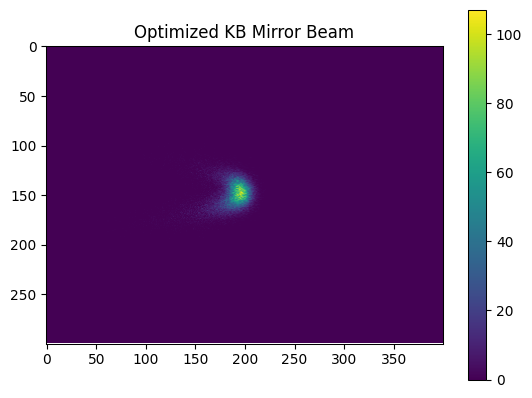
Now move the mirrors to these optimal positions and acquire an image:
from bluesky.plans import list_scan
uid = RE(list_scan(
[det],
kbv.radius, [optimal_parameters[kbv.radius.name]],
kbh.radius, [optimal_parameters[kbh.radius.name]],
))
image = tiled_client[uid[0]]["primary/det_image"].read().squeeze()
plt.imshow(image)
plt.colorbar()
plt.title("Optimized KB Mirror Beam")
plt.show()
tiled_server.close()
What You’ve Learned#
In this tutorial, you worked through a complete Bayesian optimization workflow:
DOFs define the search space — the parameters you can control and their allowed ranges
Objectives specify your optimization goal (here: minimize FWHM for a tight focal spot)
Tracking metrics (
IMetric) let you monitor values like intensity without optimizing them directlyOutcome constraints enforce safety bounds on tracked metrics (e.g., minimum beam intensity)
Evaluation functions extract meaningful metrics from experimental data using robust techniques like marginal-profile FWHM
The Agent coordinates everything, building a surrogate model of your system and intelligently exploring the parameter space
Health checks let you diagnose optimization progress and catch issues early
These same components apply to any optimization problem: swap the simulated devices for real hardware, adjust the DOFs and objectives for your system, and write an evaluation function that extracts your metrics.
Next Steps#
Learn about custom acquisition plans for more complex measurement sequences
Explore DOF constraints to encode physical limitations
See outcome constraints to enforce requirements on your results
See Also#
blop_simpackage for XRT simulated beamline control