Creating a Scan Spec#
This tutorial shows how to create Scan Specs of increasing complexity, plotting the results.
Linspace#
We’ll start with a simple one, a Linspace. If you enter the following code into an
interactive Python terminal, it should plot a graph of a 1D line:
# Example Spec
from scanspec.plot import plot_spec
from scanspec.specs import Linspace
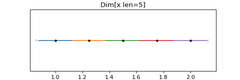
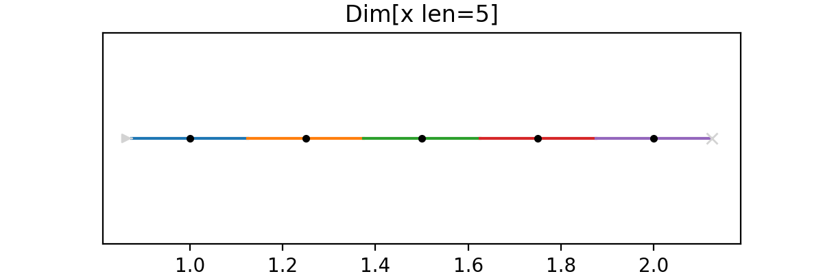
spec = Linspace("x", 1, 2, 5)
plot_spec(spec)
(Source code, png, hires.png, pdf)

This will create a Spec with 5 frames, the first centred on 1, the last centred on 2. The black dots mark the midpoints on the Path. The coloured lines mark the motion from the lower to upper bound of each frame on the Path. The grey arrowhead marks the start of the scan, and the cross marks the end.
Plotting from the commandline#
To quickly plot Scan Specs you can use the commandline client. The input is
evaluated with variables a to z defined and the output plotted.
For example, for the Linspace example above you would type:
$ scanspec plot 'Linspace(x, 1, 2, 5)'
Linspace with 2 axes#
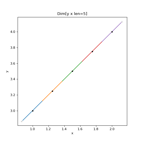
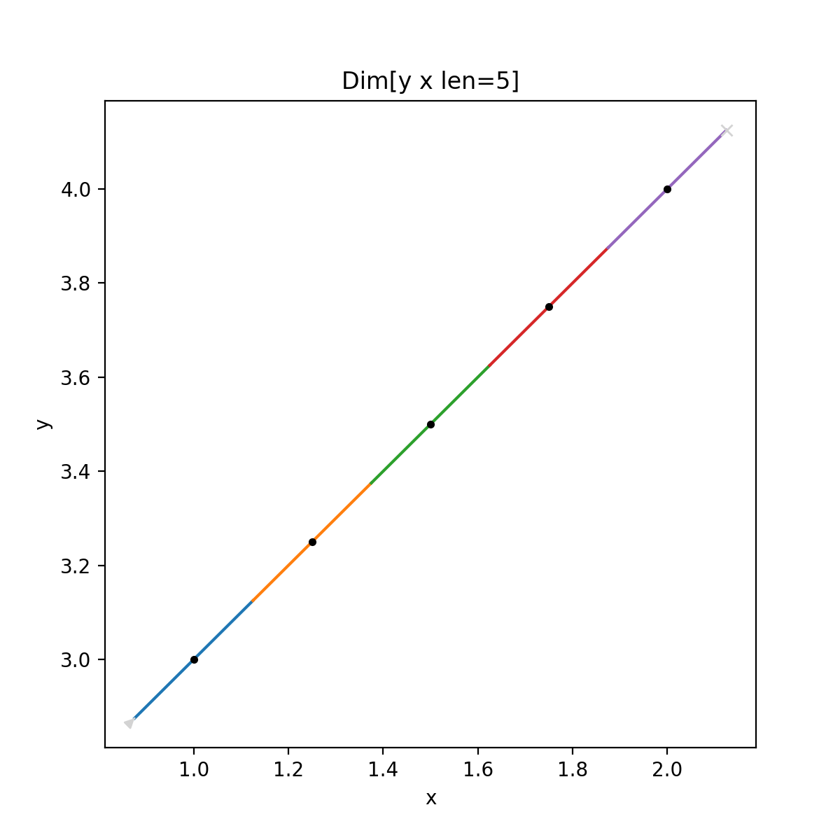
If we want to plot a Linspace in two axes, we can do this with Zip, or Spec.zip:
# Example Spec

from scanspec.plot import plot_spec
from scanspec.specs import Linspace

spec = Linspace("y", 3, 4, 5).zip(Linspace("x", 1, 2, 5))
plot_spec(spec)
(Source code, png, hires.png, pdf)

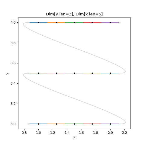
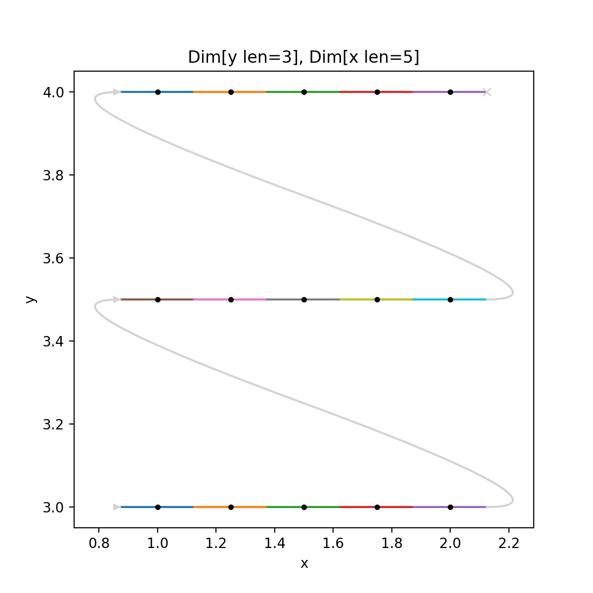
Grid#
We can make a grid by creating the Product of 2 Linspaces with the * operator:
# Example Spec

from scanspec.plot import plot_spec
from scanspec.specs import Linspace

spec = Linspace("y", 3, 4, 3) * Linspace("x", 1, 2, 5)
plot_spec(spec)
(Source code, png, hires.png, pdf)

The plot shows grey arrowed lines marking the turnarounds. These are added by the plotting function as an indication of what a scanning program might do between two disjoint frames, it is not a guarantee of the path that will be taken.
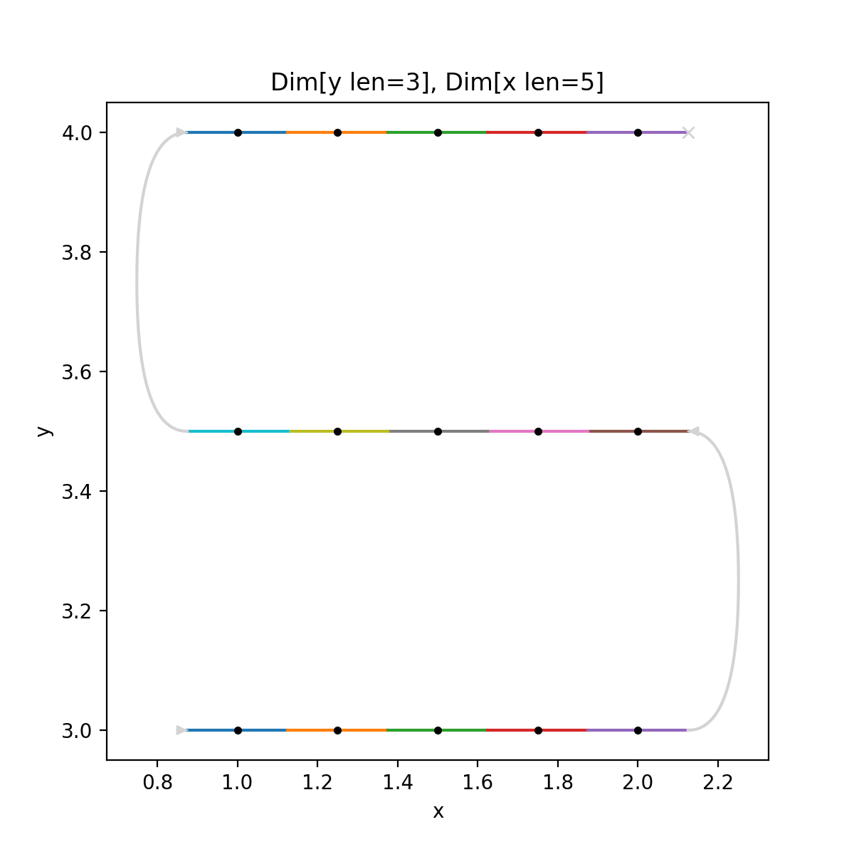
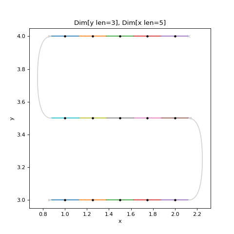
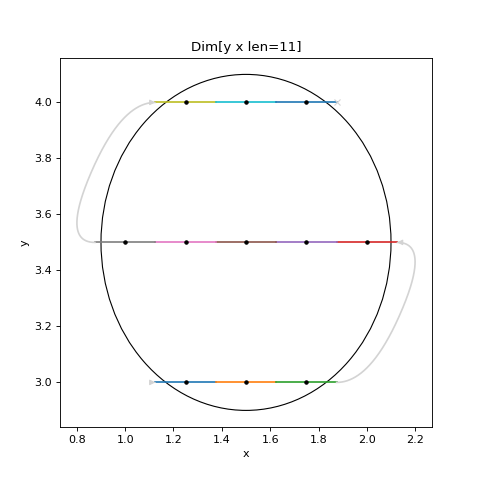
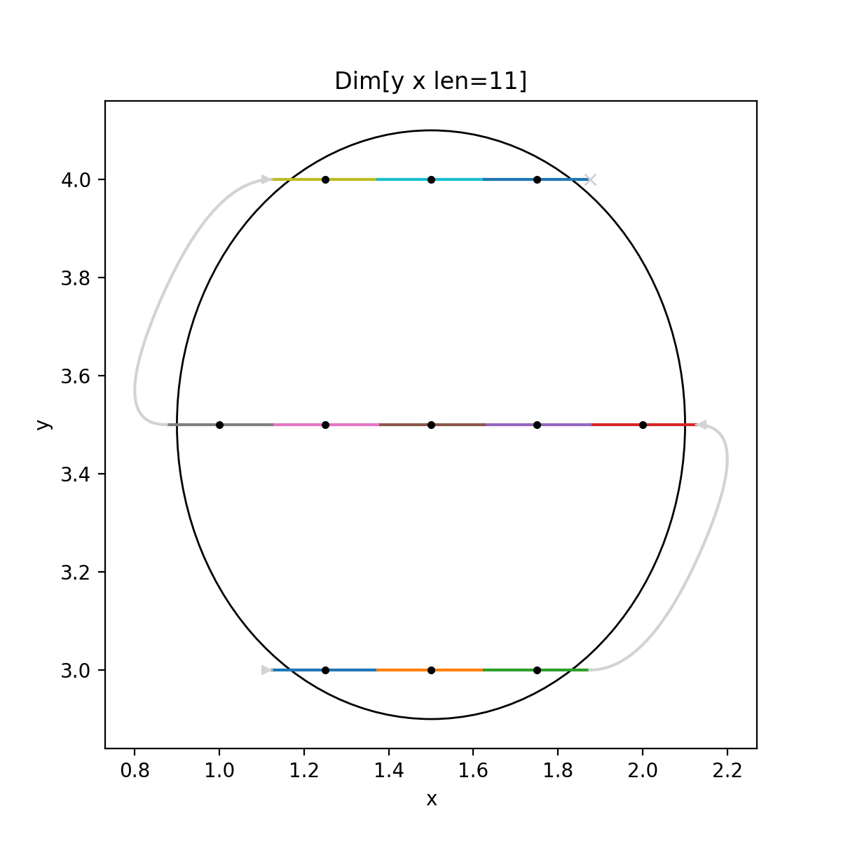
Snaked Grid#
We can Snake a Spec with the ~ operator. If we apply this to the inner
Spec of our grid we get:
# Example Spec

from scanspec.plot import plot_spec
from scanspec.specs import Linspace

spec = Linspace("y", 3, 4, 3) * ~Linspace("x", 1, 2, 5)
plot_spec(spec)
(Source code, png, hires.png, pdf)
Snaked Regions#
We can construct an Ellipse or a Polygon with a grid or a snaked grid
by passing the optional parameter snake.
For example:
# Example Spec

from scanspec.plot import plot_spec
from scanspec.specs import Ellipse

spec = Ellipse("x", 0, 1, 0.1, "y", 5, 10, 0.5, snake=True)
plot_spec(spec)
(Source code, png, hires.png, pdf)

Conclusion#
This tutorial has demonstrated some Specs and combinations of them. From here you may like to read How to Iterate a Spec to see how a scanning system could use these Specs and How to Serialize and Deserialize a Spec to see how you might send one to such a scanning system.