Your first Scipy optimization with Blop#
In this tutorial, you will learn the three core concepts of Blop: DOFs (the parameters you can adjust), objectives (what you want to optimize), and the Agent (which coordinates the optimization). We’ll optimize a simple mathematical function using simulated devices—the same patterns apply to real hardware.
Setup#
First, let’s import what we need and start the data infrastructure:
import logging
import time
from typing import Any

from bluesky.protocols import HasHints, HasParent, Hints, NamedMovable, Readable, Status
from bluesky.run_engine import RunEngine
from bluesky_tiled_plugins import TiledWriter
from tiled.client import from_uri
from tiled.client.container import Container
from tiled.server import SimpleTiledServer

from blop.scipy import SCP, ScipyCFG, Objective, RangeDOF, Scipy

# Suppress noisy logs from httpx
logging.getLogger("httpx").setLevel(logging.WARNING)
# Start a local Tiled server for data storage
tiled_server = SimpleTiledServer()

# Set up the Bluesky RunEngine and connect it to Tiled
RE = RunEngine({})
tiled_client = from_uri(tiled_server.uri)
tiled_writer = TiledWriter(tiled_client)
RE.subscribe(tiled_writer)
0
Creating simulated devices#
Bluesky controls devices through protocols. For this tutorial, we create simple simulated “movable” devices. In real experiments, you would use Ophyd devices or similar—the code below is just boilerplate to simulate hardware:
class AlwaysSuccessfulStatus(Status):
    def add_callback(self, callback) -> None:
        callback(self)

    def exception(self, timeout=0.0):
        return None

    @property
    def done(self) -> bool:
        return True

    @property
    def success(self) -> bool:
        return True


class ReadableSignal(Readable, HasHints, HasParent):
    def __init__(self, name: str) -> None:
        self._name = name
        self._value = 0.0

    @property
    def name(self) -> str:
        return self._name

    @property
    def hints(self) -> Hints:
        return {"fields": [self._name], "dimensions": [], "gridding": "rectilinear"}

    @property
    def parent(self) -> Any | None:
        return None

    def read(self):
        return {self._name: {"value": self._value, "timestamp": time.time()}}

    def describe(self):
        return {self._name: {"source": self._name, "dtype": "number", "shape": []}}


class MovableSignal(ReadableSignal, NamedMovable):
    def __init__(self, name: str, initial_value: float = 0.0) -> None:
        super().__init__(name)
        self._value: float = initial_value

    def set(self, value: float) -> Status:
        self._value = value
        return AlwaysSuccessfulStatus()
Defining DOFs and objectives#
DOFs (degrees of freedom) are the parameters the optimizer can adjust. Objectives are what you want to optimize. Here we define two DOFs (x1 and x2) that can range from -5 to 5, and one objective (the Himmelblau function) that we want to minimize:
x1 = MovableSignal("x1", initial_value=0.1)
x2 = MovableSignal("x2", initial_value=0.23)

dofs = [
    RangeDOF(actuator=x1, bounds=(-5, 5), parameter_type="float"),
    RangeDOF(actuator=x2, bounds=(-5, 5), parameter_type="float"),
]
objectives = [
    Objective(name="himmelblau_2d", minimize=True),
]
sensors = []
Writing the evaluation function#
The evaluation function computes objective values from experimental data. Blop passes it the uid returned by the acquisition plan and the suggestions that were tried. This tutorial uses the default acquisition plan, so the uid is a Bluesky run UID and blop_acquisition_order associates measurements with outcomes.
from collections.abc import Mapping, Sequence

class Himmelblau2DEvaluation:
    def __init__(self, tiled_client: Container):
        self.tiled_client = tiled_client

    def __call__(self, uid: str, suggestions: Sequence[Mapping]) -> Sequence[Mapping]:
        run = self.tiled_client[uid]
        outcomes = []
        acquisition_order = run.start["blop_acquisition_order"]
        x1_data = run["primary/x1"].read()
        x2_data = run["primary/x2"].read()

        for index, suggestion_id in enumerate(acquisition_order):
            x1 = x1_data[index]
            x2 = x2_data[index]
            # Himmelblau function: has four global minima where value = 0
            outcomes.append({"himmelblau_2d": (x1**2 + x2 - 11) ** 2 + (x1 + x2**2 - 7) ** 2, "_id": suggestion_id})

        return outcomes
Running the optimization#
The Agent brings everything together. Create one with your DOFs, objectives, and evaluation function, then run the optimization:
agent = Scipy.Agent(
    sensors=sensors,
    dofs=dofs,
    objectives=objectives,
    evaluation_function=Himmelblau2DEvaluation(tiled_client=tiled_client),
    name="simple-experiment",
    description="A simple experiment optimizing the Himmelblau function",
)

RE(agent.optimize(10))
╭───────────────────────────────────────────────── Optimization ──────────────────────────────────────────────────╮
│ Optimizer  InteractiveOptimizer                                                                                 │
│ Actuators  x1, x2                                                                                               │
│ Sensors    N/A                                                                                                  │
│ Iterations 10                                                                                                   │
│ Run UID    76997f17-1b9b-4fcd-8e01-3b7d30782178                                                                 │
╰─────────────────────────────────────────────────────────────────────────────────────────────────────────────────╯
┏━━━━━━━━━━━━━━━━━━━━━━━━━━━━┳━━━━━━━━━━━━━━━━━━━━━━━━━━━━┳━━━━━━━━━━━━━━━━━━━━━━━━━━━┳━━━━━━━━━━━━━━━━━━━━━━━━━━━┓
┃ Suggestion ID              ┃ x1                         ┃ x2                        ┃ himmelblau_2d             ┃
┡━━━━━━━━━━━━━━━━━━━━━━━━━━━━╇━━━━━━━━━━━━━━━━━━━━━━━━━━━━╇━━━━━━━━━━━━━━━━━━━━━━━━━━━╇━━━━━━━━━━━━━━━━━━━━━━━━━━━┩
└────────────────────────────┴────────────────────────────┴───────────────────────────┴───────────────────────────┘
┃                            ┃                            ┃                           ┃                           ┃
┃ 0                          ┃                          0 ┃                         0 ┃                       170 ┃
┡────────────────────────────╇────────────────────────────╇───────────────────────────╇───────────────────────────┩
┃                            ┃                            ┃                           ┃                           ┃
┃ 1                          ┃                      1e-08 ┃                         0 ┃                       170 ┃
┡────────────────────────────╇────────────────────────────╇───────────────────────────╇───────────────────────────┩
┃                            ┃                            ┃                           ┃                           ┃
┃ 2                          ┃                          0 ┃                     1e-08 ┃                       170 ┃
┡────────────────────────────╇────────────────────────────╇───────────────────────────╇───────────────────────────┩
┃                            ┃                            ┃                           ┃                           ┃
┃ 3                          ┃                          5 ┃                         5 ┃                       890 ┃
┡────────────────────────────╇────────────────────────────╇───────────────────────────╇───────────────────────────┩
┃                            ┃                            ┃                           ┃                           ┃
┃ 4                          ┃                          5 ┃                         5 ┃                       890 ┃
┡────────────────────────────╇────────────────────────────╇───────────────────────────╇───────────────────────────┩
──────────────────────────────────────────────── Iteration 5 / 10 ─────────────────────────────────────────────────
  himmelblau_2d  min: 170  max: 890  mean: 458
  (5 pts sampled)
───────────────────────────────────────────────────────────────────────────────────────────────────────────────────
┃                            ┃                            ┃                           ┃                           ┃
┃ 5                          ┃                          5 ┃                         5 ┃                       890 ┃
┡────────────────────────────╇────────────────────────────╇───────────────────────────╇───────────────────────────┩
┃                            ┃                            ┃                           ┃                           ┃
┃ 6                          ┃                    1.51545 ┃                   1.51545 ┃                   61.8302 ┃
┡────────────────────────────╇────────────────────────────╇───────────────────────────╇───────────────────────────┩
┃                            ┃                            ┃                           ┃                           ┃
┃ 7                          ┃                    1.51545 ┃                   1.51545 ┃                   61.8302 ┃
┡────────────────────────────╇────────────────────────────╇───────────────────────────╇───────────────────────────┩
┃                            ┃                            ┃                           ┃                           ┃
┃ 8                          ┃                    1.51545 ┃                   1.51545 ┃                   61.8302 ┃
┡────────────────────────────╇────────────────────────────╇───────────────────────────╇───────────────────────────┩
┃                            ┃                            ┃                           ┃                           ┃
┃ 9                          ┃                    3.25772 ┃                   3.25772 ┃                   55.4432 ┃
┡────────────────────────────╇────────────────────────────╇───────────────────────────╇───────────────────────────┩
──────────────────────────────────────────────── Iteration 10 / 10 ────────────────────────────────────────────────
  himmelblau_2d  min: 55.4432  max: 890  mean: 342.093
  (10 pts sampled)
───────────────────────────────────────────────────────────────────────────────────────────────────────────────────
                          Summary Statistics
┏━━━━━━━━━━━━━━━┳━━━━━━━━━┳━━━━━━━━━┳━━━━━┳━━━━━━━━━┳━━━━━━━━━┳━━━━━━━┓
┃ Name          ┃ Type    ┃     Min ┃ Max ┃    Mean ┃     Std ┃ Count ┃
┡━━━━━━━━━━━━━━━╇━━━━━━━━━╇━━━━━━━━━╇━━━━━╇━━━━━━━━━╇━━━━━━━━━╇━━━━━━━┩
│ x1            │ param   │       0 │   5 │ 2.28041 │ 2.12132 │    10 │
│ x2            │ param   │       0 │   5 │ 2.28041 │ 2.12132 │    10 │
│ himmelblau_2d │ outcome │ 55.4432 │ 890 │ 342.093 │ 381.119 │    10 │
└───────────────┴─────────┴─────────┴─────┴─────────┴─────────┴───────┘
────────────────────────────────────────────── Optimization Complete ──────────────────────────────────────────────
('76997f17-1b9b-4fcd-8e01-3b7d30782178',
 'f7063772-03d1-41aa-bde4-e682f210ee75',
 '1a0842f2-133a-43ef-a0f9-f47b16ad32a7',
 '15880526-c82b-4b1a-a970-1394b386a141',
 'c7e3753b-57eb-449e-bf17-3040f66b4d1e',
 '13dab3eb-0316-4cd6-8a13-747a05c671e5',
 'c207ba18-c220-400f-a759-b1c10c2f4bca',
 '1d862963-f406-47fd-906c-022df6b7edee',
 '82dd068a-125d-406d-a0c0-6b38087decd3',
 '931e1842-b4ec-43ba-b319-a1abd48a8b18',
 '1ef05549-d051-440a-89dd-ef448bbfdbf0')
Configuring the optimization#
Sometimes a default Agent optimization may not do all that you’d like. We expose a configuration object called ScipyCFG and a pure scipy interface so that the classic parameters of scipy minimize can be tweaked (and some multipoint sampling can be used).
config = ScipyCFG(dofs=dofs, objective=objectives[0], optimizer=SCP.DUAL_ANNEALING, threads=4, max_iter=2, eps=0.1)
agent = Scipy(
    sensors=sensors,
    config=config,
    evaluation_function=Himmelblau2DEvaluation(tiled_client=tiled_client),
    name="test_experiment",
)
res_uid = RE(agent.optimize(20, n_points=2))
╭───────────────────────────────────────────────── Optimization ──────────────────────────────────────────────────╮
│ Optimizer  InteractiveOptimizer                                                                                 │
│ Actuators  x1, x2                                                                                               │
│ Sensors    N/A                                                                                                  │
│ Iterations 20  Points/iter 2                                                                                    │
│ Run UID    efda92a2-6d3c-4cf3-9ade-56f31351f4a2                                                                 │
╰─────────────────────────────────────────────────────────────────────────────────────────────────────────────────╯
┏━━━━━━━━━━━━━━━━━━━━━━━━━━━━┳━━━━━━━━━━━━━━━━━━━━━━━━━━━━┳━━━━━━━━━━━━━━━━━━━━━━━━━━━┳━━━━━━━━━━━━━━━━━━━━━━━━━━━┓
┃ Suggestion ID              ┃ x1                         ┃ x2                        ┃ himmelblau_2d             ┃
┡━━━━━━━━━━━━━━━━━━━━━━━━━━━━╇━━━━━━━━━━━━━━━━━━━━━━━━━━━━╇━━━━━━━━━━━━━━━━━━━━━━━━━━━╇━━━━━━━━━━━━━━━━━━━━━━━━━━━┩
└────────────────────────────┴────────────────────────────┴───────────────────────────┴───────────────────────────┘
┃                            ┃                            ┃                           ┃                           ┃
┃ 0                          ┃                          0 ┃                         0 ┃                       170 ┃
┡────────────────────────────╇────────────────────────────╇───────────────────────────╇───────────────────────────┩
┃                            ┃                            ┃                           ┃                           ┃
┃ 1                          ┃                  0.0252218 ┃                 0.0252218 ┃                    169.07 ┃
┡────────────────────────────╇────────────────────────────╇───────────────────────────╇───────────────────────────┩
┃                            ┃                            ┃                           ┃                           ┃
┃ 2                          ┃                   -1.75436 ┃                  -1.75436 ┃                    125.86 ┃
┡────────────────────────────╇────────────────────────────╇───────────────────────────╇───────────────────────────┩
┃                            ┃                            ┃                           ┃                           ┃
┃ 3                          ┃                    3.77717 ┃                  -1.75436 ┃                   2.30917 ┃
┡────────────────────────────╇────────────────────────────╇───────────────────────────╇───────────────────────────┩
/home/runner/work/blop/blop/.pixi/envs/docs/lib/python3.13/site-packages/scipy/optimize/_dual_annealing.py:434: OptimizeWarning: Unknown solver options: max_iter
  mres = self.minimizer(self.func_wrapper.fun, x, **self.kwargs)
┃                            ┃                            ┃                           ┃                           ┃
┃ 4                          ┃                    3.77717 ┃                    3.3523 ┃                   108.057 ┃
┡────────────────────────────╇────────────────────────────╇───────────────────────────╇───────────────────────────┩
──────────────────────────────────────────────── Iteration 5 / 20 ─────────────────────────────────────────────────
  himmelblau_2d  min: 2.30917  max: 170  mean: 115.059
  (5 pts sampled)
───────────────────────────────────────────────────────────────────────────────────────────────────────────────────
┃                            ┃                            ┃                           ┃                           ┃
┃ 5                          ┃                    3.77717 ┃                  -1.75436 ┃                   2.30917 ┃
┡────────────────────────────╇────────────────────────────╇───────────────────────────╇───────────────────────────┩
┃                            ┃                            ┃                           ┃                           ┃
┃ 6                          ┃                    3.87717 ┃                  -1.75436 ┃                   5.19173 ┃
┡────────────────────────────╇────────────────────────────╇───────────────────────────╇───────────────────────────┩
┃                            ┃                            ┃                           ┃                           ┃
┃ 7                          ┃                    3.77717 ┃                  -1.65436 ┃                   2.83679 ┃
┡────────────────────────────╇────────────────────────────╇───────────────────────────╇───────────────────────────┩
┃                            ┃                            ┃                           ┃                           ┃
┃ 8                          ┃                         -5 ┃                        -5 ┃                       250 ┃
┡────────────────────────────╇────────────────────────────╇───────────────────────────╇───────────────────────────┩
┃                            ┃                            ┃                           ┃                           ┃
┃ 10                         ┃                       -4.9 ┃                        -5 ┃                    235.77 ┃
┡────────────────────────────╇────────────────────────────╇───────────────────────────╇───────────────────────────┩
──────────────────────────────────────────────── Iteration 9 / 20 ─────────────────────────────────────────────────
  himmelblau_2d  min: 2.30917  max: 250  mean: 107.14
  (10 pts sampled)
───────────────────────────────────────────────────────────────────────────────────────────────────────────────────
┃                            ┃                            ┃                           ┃                           ┃
┃ 9                          ┃                         -5 ┃                      -4.9 ┃                    227.05 ┃
┡────────────────────────────╇────────────────────────────╇───────────────────────────╇───────────────────────────┩
┃                            ┃                            ┃                           ┃                           ┃
┃ 11                         ┃                   0.327589 ┃                  -3.02995 ┃                   200.131 ┃
┡────────────────────────────╇────────────────────────────╇───────────────────────────╇───────────────────────────┩
┃                            ┃                            ┃                           ┃                           ┃
┃ 12                         ┃                   0.427589 ┃                  -3.02995 ┃                   198.545 ┃
┡────────────────────────────╇────────────────────────────╇───────────────────────────╇───────────────────────────┩
┃                            ┃                            ┃                           ┃                           ┃
┃ 13                         ┃                   0.327589 ┃                  -2.92995 ┃                   194.722 ┃
┡────────────────────────────╇────────────────────────────╇───────────────────────────╇───────────────────────────┩
┃                            ┃                            ┃                           ┃                           ┃
┃ 14                         ┃                    3.48865 ┃                  -1.86105 ┃                  0.478894 ┃
┡────────────────────────────╇────────────────────────────╇───────────────────────────╇───────────────────────────┩
──────────────────────────────────────────────── Iteration 12 / 20 ────────────────────────────────────────────────
  himmelblau_2d  min: 0.478894  max: 250  mean: 126.155
  (15 pts sampled)
───────────────────────────────────────────────────────────────────────────────────────────────────────────────────
┃                            ┃                            ┃                           ┃                           ┃
┃ 15                         ┃                    3.58865 ┃                  -1.86105 ┃                0.00302061 ┃
┡────────────────────────────╇────────────────────────────╇───────────────────────────╇───────────────────────────┩
┃                            ┃                            ┃                           ┃                           ┃
┃ 16                         ┃                    3.48865 ┃                  -1.76105 ┃                  0.516684 ┃
┡────────────────────────────╇────────────────────────────╇───────────────────────────╇───────────────────────────┩
┃                            ┃                            ┃                           ┃                           ┃
┃ 17                         ┃                    3.52772 ┃                  -1.85685 ┃                  0.170375 ┃
┡────────────────────────────╇────────────────────────────╇───────────────────────────╇───────────────────────────┩
┃                            ┃                            ┃                           ┃                           ┃
┃ 18                         ┃                    3.52772 ┃                  -1.75685 ┃                  0.246182 ┃
┡────────────────────────────╇────────────────────────────╇───────────────────────────╇───────────────────────────┩
┃                            ┃                            ┃                           ┃                           ┃
┃ 19                         ┃                    3.62772 ┃                  -1.85685 ┃                 0.0978293 ┃
┡────────────────────────────╇────────────────────────────╇───────────────────────────╇───────────────────────────┩
──────────────────────────────────────────────── Iteration 15 / 20 ────────────────────────────────────────────────
  himmelblau_2d  min: 0.00302061  max: 250  mean: 94.6683
  (20 pts sampled)
───────────────────────────────────────────────────────────────────────────────────────────────────────────────────
┃                            ┃                            ┃                           ┃                           ┃
┃ 20                         ┃                    3.53472 ┃                  -1.86493 ┃                   0.13757 ┃
┡────────────────────────────╇────────────────────────────╇───────────────────────────╇───────────────────────────┩
┃                            ┃                            ┃                           ┃                           ┃
┃ 21                         ┃                    3.63472 ┃                  -1.86493 ┃                  0.132595 ┃
┡────────────────────────────╇────────────────────────────╇───────────────────────────╇───────────────────────────┩
┃                            ┃                            ┃                           ┃                           ┃
┃ 22                         ┃                    3.53472 ┃                  -1.76493 ┃                  0.195974 ┃
┡────────────────────────────╇────────────────────────────╇───────────────────────────╇───────────────────────────┩
┃                            ┃                            ┃                           ┃                           ┃
┃ 23                         ┃                    3.53822 ┃                  -1.88046 ┃                  0.136158 ┃
┡────────────────────────────╇────────────────────────────╇───────────────────────────╇───────────────────────────┩
┃                            ┃                            ┃                           ┃                           ┃
┃ 24                         ┃                    3.53822 ┃                  -1.78046 ┃                  0.153457 ┃
┡────────────────────────────╇────────────────────────────╇───────────────────────────╇───────────────────────────┩
──────────────────────────────────────────────── Iteration 19 / 20 ────────────────────────────────────────────────
  himmelblau_2d  min: 0.00302061  max: 250  mean: 75.7648
  (25 pts sampled)
───────────────────────────────────────────────────────────────────────────────────────────────────────────────────
┃                            ┃                            ┃                           ┃                           ┃
┃ 25                         ┃                    3.63822 ┃                  -1.88046 ┃                  0.157289 ┃
┡────────────────────────────╇────────────────────────────╇───────────────────────────╇───────────────────────────┩
┃                            ┃                            ┃                           ┃                           ┃
┃ 26                         ┃                    3.53669 ┃                  -1.88617 ┃                   0.15178 ┃
┡────────────────────────────╇────────────────────────────╇───────────────────────────╇───────────────────────────┩
                              Summary Statistics
┏━━━━━━━━━━━━━━━┳━━━━━━━━━┳━━━━━━━━━━━━┳━━━━━━━━━┳━━━━━━━━━━┳━━━━━━━━━┳━━━━━━━┓
┃ Name          ┃ Type    ┃        Min ┃     Max ┃     Mean ┃     Std ┃ Count ┃
┡━━━━━━━━━━━━━━━╇━━━━━━━━━╇━━━━━━━━━━━━╇━━━━━━━━━╇━━━━━━━━━━╇━━━━━━━━━╇━━━━━━━┩
│ x1            │ param   │         -5 │ 3.87717 │  1.83867 │ 2.92574 │    27 │
│ x2            │ param   │         -5 │  3.3523 │ -1.96519 │ 1.60349 │    27 │
│ himmelblau_2d │ outcome │ 0.00302061 │     250 │  70.1641 │ 95.9078 │    27 │
└───────────────┴─────────┴────────────┴─────────┴──────────┴─────────┴───────┘
────────────────────────────────────────────── Optimization Complete ──────────────────────────────────────────────
Viewing the results#
Scipy is a local optimizer so it doesn’t have internal point tracking, but we can to grab it from our datastore.
import numpy as np
import matplotlib.pyplot as plt
import pandas as pd

res_client = tiled_client[res_uid[0]]
data = res_client["primary"].read().to_dataframe()

fig, ax = plt.subplots(figsize=(12, 8))

xb, yb = np.random.uniform(-5, 5, (2, 1000))
ax.tripcolor(xb, yb, (xb**2 + yb - 11) ** 2 + (xb + yb**2 - 7) ** 2, shading="gouraud")

ps = ax.scatter(data.x1, data.x2, marker='+', c=range(len(data.x1)), cmap="plasma", s=50)
plt.colorbar(ps).set_label("sample index")
plt.title("Visualizing Scipy's traversal of Himmelblau")
Text(0.5, 1.0, "Visualizing Scipy's traversal of Himmelblau")
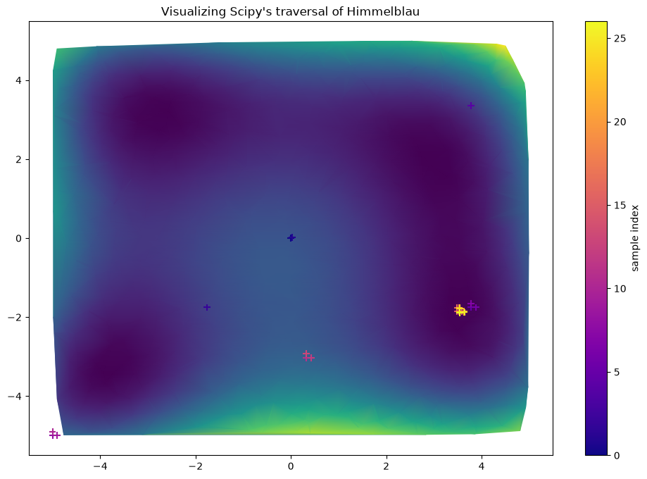
Seeing the sample history
data
| iteration | acquisition_uid | suggestion_ids | himmelblau_2d | x1 | x2 | |
|---|---|---|---|---|---|---|
| time | ||||||
| 1.792787e+09 | 0 | 915c8a23-3f68-48af-a6cf-55d843986012 | 0 | 170.000000 | 0.000000 | 0.000000 |
| 1.792787e+09 | 1 | 8259d4c9-a582-42ae-94ff-3eea8ab55d62 | 1 | 169.070453 | 0.025222 | 0.025222 |
| 1.792787e+09 | 2 | a35bc3b7-9863-4666-9d36-8a2bbb6a5819 | 2 | 125.860021 | -1.754357 | -1.754357 |
| 1.792787e+09 | 3 | f7e6a836-f30a-437b-86db-7e192778c7d1 | 3 | 2.309175 | 3.777170 | -1.754357 |
| 1.792787e+09 | 4 | 37f7fb18-e057-4436-85b7-960e16a8d065 | 4 | 108.056660 | 3.777170 | 3.352298 |
| 1.792787e+09 | 5 | 5a47f130-fb16-40e1-b4e8-1d80e5510a4f | 5 | 2.309175 | 3.777170 | -1.754357 |
| 1.792787e+09 | 6 | f14396e2-5600-4d7d-a037-7eb0dc7da2de | 6 | 5.191731 | 3.877170 | -1.754357 |
| 1.792787e+09 | 6 | f14396e2-5600-4d7d-a037-7eb0dc7da2de | 7 | 2.836794 | 3.777170 | -1.654357 |
| 1.792787e+09 | 7 | 3cec6a17-8c5b-4fbb-bef5-9c03f44438b2 | 8 | 250.000000 | -5.000000 | -5.000000 |
| 1.792787e+09 | 8 | 70318097-897c-43fb-bf2d-94b87e5b5f14 | 10 | 235.770100 | -4.900000 | -5.000000 |
| 1.792787e+09 | 8 | 70318097-897c-43fb-bf2d-94b87e5b5f14 | 9 | 227.050100 | -5.000000 | -4.900000 |
| 1.792787e+09 | 9 | a111b95d-4963-4520-b2a5-a7046474d0da | 11 | 200.130854 | 0.327589 | -3.029951 |
| 1.792787e+09 | 10 | 38443ace-56a7-483f-91fc-501f8a026db5 | 12 | 198.545382 | 0.427589 | -3.029951 |
| 1.792787e+09 | 10 | 38443ace-56a7-483f-91fc-501f8a026db5 | 13 | 194.721812 | 0.327589 | -2.929951 |
| 1.792787e+09 | 11 | d86e1b56-6d21-4ad0-870b-2ae6c664e0ac | 14 | 0.478894 | 3.488650 | -1.861047 |
| 1.792787e+09 | 12 | fc47c53b-b91c-4aa5-bb63-93fd44136892 | 15 | 0.003021 | 3.588650 | -1.861047 |
| 1.792787e+09 | 12 | fc47c53b-b91c-4aa5-bb63-93fd44136892 | 16 | 0.516684 | 3.488650 | -1.761047 |
| 1.792787e+09 | 13 | 91ef328f-76c3-4c1d-bbac-cc5c6e9f90d9 | 17 | 0.170375 | 3.527720 | -1.856850 |
| 1.792787e+09 | 14 | 79ff5dec-7c77-4224-9bf7-4a75b52461c0 | 18 | 0.246182 | 3.527720 | -1.756850 |
| 1.792787e+09 | 14 | 79ff5dec-7c77-4224-9bf7-4a75b52461c0 | 19 | 0.097829 | 3.627720 | -1.856850 |
| 1.792787e+09 | 15 | d177b15c-9167-490e-aa7c-f1ee3c3a4c45 | 20 | 0.137570 | 3.534720 | -1.864934 |
| 1.792787e+09 | 16 | 501968b1-fe44-4ed2-82aa-e0d19d36c297 | 21 | 0.132595 | 3.634720 | -1.864934 |
| 1.792787e+09 | 16 | 501968b1-fe44-4ed2-82aa-e0d19d36c297 | 22 | 0.195974 | 3.534720 | -1.764934 |
| 1.792787e+09 | 17 | fc0b2046-608b-425f-83f0-307b52396495 | 23 | 0.136158 | 3.538224 | -1.880459 |
| 1.792787e+09 | 18 | 211cac6a-a66f-43f8-9979-0f4b430947b7 | 24 | 0.153457 | 3.538224 | -1.780459 |
| 1.792787e+09 | 18 | 211cac6a-a66f-43f8-9979-0f4b430947b7 | 25 | 0.157289 | 3.638224 | -1.880459 |
| 1.792787e+09 | 19 | 8823fc87-0147-4bc6-b959-7895662b8620 | 26 | 0.151780 | 3.536689 | -1.886167 |
print(agent.get_best_points())
[25, {'x1': np.float64(3.536688553666474), 'x2': np.float64(-1.8861671423810296)}, {'himmelblau_2d': np.float64(0.1361580929332407)}]
The Himmelblau function has four global minima (all with value 0). The summarize output shows which one(s) the optimizer found.
What you learned#
You now understand the three core concepts of Blop:
DOFs: The parameters the optimizer adjusts (here,
x1andx2with bounds)Objectives: What you’re optimizing (here, minimizing the Himmelblau function)
Agent: Coordinates the optimization loop between Bluesky and the evaluation function
Next steps#
For a more comprehensive tutorial with multiple objectives and diagnostic tools, see Optimizing KB Mirrors.