hkl_soleil E6C psi axis#
Show how to set, compute, and scan \(\psi\) with the E6C diffractometer
geometry. Use the hkl_soleil solver. Scan
\(\psi\) at fixed \(Q\) and \(hkl_2\).
Virtual axes, such as \(\psi\), are features provided by the solver as extras. Extras are not necessarily available in every solver. Consult the solver documentation for details.
NOTE
ⓘ The demonstrations below rely on features provided by the
hkl_soleilsolver.
Concise Summary#
Define an E6C diffractometer object using
hklcomputation engine (the default).Add a sample.
Add two known reflections, and compute its \(UB\) matrix
Set \(\psi\)
Use the
"psi_constant_vertical"mode.Make a dictionary with \(hkl_2\) and \(\psi\).
Finally, compute the real-space position at \(hkl\).
Compute \(\psi\)
Create a second E6C diffractometer object using the
"psi"computation engine.Copy the \(UB\) matrix from the
e6c_hkldiffractometer.Set \(hkl_2\). (Since these are simulators, copy the real-space motor positions.)
Show the position of \(\psi\).
Scan \(\psi\)
Run the diffractometer’s custom
scan_extra()plan, specifying both \(hkl\) (aspseudos) andhkl_2(asextras).
Overview#
To work with \(\psi\) we’ll use the "hkl" engine of the E6C
geometry. To compute \(\psi\) we’ll use the
"psi" engine. This table summarizes our use:
engine |
how it is used |
|---|---|
|
work in reciprocal-space coordinates \(h, k, l\) |
|
compute the \(\psi\) rotation angle (not for operations) |
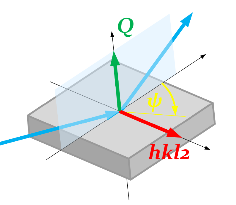
\(\psi\) is the rotation of reference vector \(hkl_2\) perpendicular to scattering
vector Q:
color |
description |
|---|---|
blue |
incident and exit X-ray beams |
green |
scattering vector (\(Q\)) |
red |
reference vector (\(hkl_2\)) |
yellow |
rotation (\(\psi\)) from \(hkl_2\) around \(Q\) |
black |
principle cartesian axes |
gray |
sample |
Steps#
With the
"hkl"engine:Orient a crystalline sample with the
"hkl"engine.Define the azimuthal reflection \(h_2, k_2, l_2\) and a \(\psi\) rotation.
Position the diffractometer for the \(h, k, l\) reflection.
With the
"psi"engine:Copy sample and orientation information from the
"hkl"instance.Copy position information:
This step is necessary since this notebook uses simulated motors.
Diffractometers using EPICS motors will do this automatically.
Compute
psi.Compare the computed
psivalue with the value set with the"hkl"instance.
Scan \(\psi\) at fixed \(Q\) and \(hkl_2\).
Setup E6C Simulators#
Create instances of (simulated) E6C for the "hkl" and "psi" solver engines.
The hklpy2.creator() function creates both.
import hklpy2

e6c_hkl = hklpy2.creator(
    name="e6c_hkl",
    geometry="E6C",
    solver="hkl_soleil",
    solver_kwargs={"engine": "hkl"},
)
e6c_psi = hklpy2.creator(
    name="e6c_psi",
    geometry="E6C",
    solver="hkl_soleil",
    solver_kwargs={"engine": "psi"},
)
Show the different calculation engines available for the E6C geometry.
print(f"{e6c_hkl.core.solver.engines=}")
e6c_hkl.core.solver.engines=['hkl', 'psi', 'q2', 'qper_qpar', 'tth2', 'incidence', 'emergence']
NOTE
ⓘ The
solverworks at a lower level than ophyd. All the code and structures used by a solver are pure Python code (or calls from Python to lower level libraries.)
Show the different operation modes available with each engine for the E6C geometry.
The hkl engine has a "psi_constant_vertical" mode that can be used to calculate reals given some fixed parameters (UB, wavelength, $(hkl)$, $(hkl)_2$, $\psi$). The psi engine has only one mode.
print(f"{e6c_hkl.core.modes=}")
print(f"{e6c_psi.core.modes=}")
e6c_hkl.core.modes=['bissector_vertical', 'constant_omega_vertical', 'constant_chi_vertical', 'constant_phi_vertical', 'lifting_detector_phi', 'lifting_detector_omega', 'lifting_detector_mu', 'double_diffraction_vertical', 'bissector_horizontal', 'double_diffraction_horizontal', 'psi_constant_vertical', 'psi_constant_horizontal', 'constant_mu_horizontal']
e6c_psi.core.modes=['psi_vertical']
Show the extra axes available with each mode used by this notebook. (The extras have default values at this time.)
The psi engine has a pseudo axis "psi" that can be used to calculate $\psi$ given some fixed parameters (reals, UB, wavelength, $(hkl)$, $(hkl)_2$)
e6c_hkl.core.mode = "bissector_vertical"
print(f"{e6c_hkl.core.mode=}")
print(f"{e6c_hkl.core.extras=}")

e6c_hkl.core.mode = "psi_constant_vertical"
print(f"{e6c_hkl.core.mode=}")
print(f"{e6c_hkl.core.extras=}")

# "psi" engine has only one mode, do not need to set it
print(f"{e6c_psi.core.mode=}")
print(f"{e6c_psi.core.extras=}")
e6c_hkl.core.mode='bissector_vertical'
e6c_hkl.core.extras={}
e6c_hkl.core.mode='psi_constant_vertical'
e6c_hkl.core.extras={'h2': 0, 'k2': 0, 'l2': 0, 'psi': 0}
e6c_psi.core.mode='psi_vertical'
e6c_psi.core.extras={'h2': 0, 'k2': 0, 'l2': 0}
Define and orient a sample#
The sample for this notebook is crystalline vibranium, with a cubic lattice of exactly $2\pi$. With it mounted on oru diffractometer, we have identified two reflections which define its orientation.
import math

e6c_hkl.beam.wavelength.put(1.54)  # angstrom (8.0509 keV)

e6c_hkl.add_sample("vibranium", 2 * math.pi, digits=5)

e6c_hkl.add_reflection((4, 0, 0), (0, 29.354, 0, 2, 0, 58.71), name="r400")
e6c_hkl.add_reflection((0, 4, 0), (0, 29.354, 0, 92, 0, 58.71), name="r040")
for r in e6c_hkl.sample.reflections.order:
    print(f"{e6c_hkl.sample.reflections[r]}")
e6c_hkl.core.calc_UB(*e6c_hkl.sample.reflections.order)

print(f"{e6c_hkl.sample.UB=!r}")
print(f"{e6c_hkl.sample.U=!r}")
Reflection(name='r400', h=4, k=0, l=0)
Reflection(name='r040', h=0, k=4, l=0)
e6c_hkl.sample.UB=[[0.034882054037, 0.999391435978, -0.0], [0.0, 0.0, 1.0], [0.999391435978, -0.034882054037, -0.0]]
e6c_hkl.sample.U=[[0.034882054037, 0.999391435978, 0.0], [0.0, 0.0, 1.0], [0.999391435978, -0.034882054037, 0.0]]
Set axis constraints#
Restrict axes to a single solution branch before any motion. Using the negative branch ($\chi\leq0$, $\delta\leq0$) ensures the solver stays consistent throughout the notebook — including the later azimuthal scan of $(002)$, where alternating between branches would cause a discontinuous jump in $\varphi$.
e6c_hkl.core.constraints["mu"].limits = 0, 0
e6c_hkl.core.constraints["omega"].limits = -180, 0
e6c_hkl.core.constraints["chi"].limits = -180, 0.1  # allow chi=-90 boundary
e6c_hkl.core.constraints["phi"].limits = -180, 0
e6c_hkl.core.constraints["gamma"].limits = 0, 0
e6c_hkl.core.constraints["delta"].limits = -180, 0
print(e6c_hkl.core.constraints)
['0.0 <= mu <= 0.0 [cut=-180.0]', '-180.0 <= omega <= 0.0 [cut=-180.0]', '-180.0 <= chi <= 0.1 [cut=-180.0]', '-180.0 <= phi <= 0.0 [cut=-180.0]', '0.0 <= gamma <= 0.0 [cut=-180.0]', '-180.0 <= delta <= 0.0 [cut=-180.0]']
Move to the $(111)$ orientation#
Before moving the diffractometer, ensure you have selected the desired operating mode.
e6c_hkl.core.mode = "bissector_vertical"
e6c_hkl.move(1, 0, 0)
e6c_hkl.position, e6c_hkl.real_position
(Hklpy2DiffractometerPseudoPos(h=1.0, k=-0.0, l=0.0),
 Hklpy2DiffractometerRealPos(mu=0.0, omega=-7.0393, chi=-0.0, phi=-178.001, gamma=0.0, delta=-14.0785))
Set ${hkl}_2$ and $\psi$#
Show the extra axes available with psi_constant_vertical mode.
e6c_hkl.core.mode = "psi_constant_vertical"
print(f"{e6c_hkl.core.solver_extra_axis_names=}")
e6c_hkl.core.solver_extra_axis_names=['h2', 'k2', 'l2', 'psi']
Set azimuthal reflection ${hkl}_2 = (110)$ and $\psi=12$.
The extras are described as a Python dictionary with values for each of the parameters.
e6c_hkl.core.extras = dict(h2=1, k2=1, l2=0, psi=12)
print(f"{e6c_hkl.core.extras=}")
e6c_hkl.core.extras={'h2': 1, 'k2': 1, 'l2': 0, 'psi': 12}
Compute the real-axis motor values with the $Q=(111)$ reflection oriented and $\psi$ rotation.
p_111 = e6c_hkl.forward(1, 1, 1)
print(f"{p_111=}")
p_111=Hklpy2DiffractometerRealPos(mu=0.0, omega=-66.3916, chi=-80.2262, phi=-49.9973, gamma=0.0, delta=-24.5098)
Move each real (real-space positioner) to the computed $(111)$ reflection position p_111.
e6c_hkl.move_reals(p_111)
print(f"{e6c_hkl.position=}")
print(f"{e6c_hkl.real_position=}")
print(f"{e6c_hkl.core.extras=}")
e6c_hkl.position=Hklpy2DiffractometerPseudoPos(h=1.0, k=1.0, l=1.0)
e6c_hkl.real_position=Hklpy2DiffractometerRealPos(mu=0.0, omega=-66.3916, chi=-80.2262, phi=-49.9973, gamma=0.0, delta=-24.5098)
e6c_hkl.core.extras={'h2': 1, 'k2': 1, 'l2': 0, 'psi': 12}
Compute $\psi$ at fixed $Q$ and $hkl_2$#
We’ll use the "psi" engine to compute $\psi$, given a sample & orientation,
${hkl}_2$, and the real-space motor positions.
print(f"{e6c_psi.core.mode=}")
print(f"{e6c_psi.core.extras=}")
e6c_psi.core.mode='psi_vertical'
e6c_psi.core.extras={'h2': 0, 'k2': 0, 'l2': 0}
Same sample and lattice
e6c_psi.add_sample("vibranium", 2 * math.pi, digits=5)
Sample(name='vibranium', lattice=Lattice(a=6.28319, system='cubic'))
Copy orientation from hkl instance. Note the psi and hkl UB matrices are
not exactly equal. Equal to about 5 decimal places.)
e6c_psi.sample.UB = e6c_hkl.sample.UB

print(f"{e6c_psi.sample.UB=!r}")
print(f"{e6c_psi.sample.U=!r}")

print(f"{e6c_hkl.sample.UB=!r}")
print(f"{e6c_hkl.sample.U=!r}")
e6c_psi.sample.UB=[[0.034882054037, 0.999391435978, -0.0], [0.0, 0.0, 1.0], [0.999391435978, -0.034882054037, -0.0]]
e6c_psi.sample.U=[[1, 0, 0], [0, 1, 0], [0, 0, 1]]
e6c_hkl.sample.UB=[[0.034882054037, 0.999391435978, -0.0], [0.0, 0.0, 1.0], [0.999391435978, -0.034882054037, -0.0]]
e6c_hkl.sample.U=[[0.034882054037, 0.999391435978, 0.0], [0.0, 0.0, 1.0], [0.999391435978, -0.034882054037, 0.0]]
Set ${hkl}_2=(1, 1, 0)$. As above, describe these parameters in a Python dictionary.
e6c_psi.core.extras = dict(h2=1, k2=1, l2=0)
print(f"{e6c_psi.core.extras=}")
e6c_psi.core.extras={'h2': 1, 'k2': 1, 'l2': 0}
Set real-space axis positions from p_111 (above).
e6c_psi.move_reals(p_111)
print(f"{e6c_psi.pseudo_axis_names=}")
print(f"{e6c_psi.core.solver_pseudo_axis_names=}")
print(f"{e6c_psi.position=}")
print(f"{e6c_psi.real_position=}")
e6c_psi.pseudo_axis_names=['psi']
e6c_psi.core.solver_pseudo_axis_names=['psi']
e6c_psi.position=Hklpy2DiffractometerPseudoPos(psi=12.0)
e6c_psi.real_position=Hklpy2DiffractometerRealPos(mu=0.0, omega=-66.3916, chi=-80.2262, phi=-49.9973, gamma=0.0, delta=-24.5098)
Compare hkl and psi reports.
print(e6c_hkl)
e6c_hkl.wh()
print(e6c_psi)
e6c_psi.wh()
Hklpy2Diffractometer(prefix='', name='e6c_hkl', settle_time=0.0, timeout=None, egu='', limits=(0, 0), source='computed', read_attrs=['beam', 'beam.wavelength', 'beam.energy', 'h', 'h.readback', 'h.setpoint', 'k', 'k.readback', 'k.setpoint', 'l', 'l.readback', 'l.setpoint', 'mu', 'omega', 'chi', 'phi', 'gamma', 'delta'], configuration_attrs=['beam', 'beam.source_type', 'beam.wavelength_units', 'beam.wavelength_deadband', 'beam.energy_units', 'h', 'k', 'l'], concurrent=True)
wavelength=1.54
pseudos: h=1.0, k=1.0, l=1.0
reals: mu=0, omega=-66.3916, chi=-80.2262, phi=-49.9973, gamma=0, delta=-24.5098
extras: h2=1 k2=1 l2=0 psi=12
Hklpy2Diffractometer(prefix='', name='e6c_psi', settle_time=0.0, timeout=None, egu='', limits=(0, 0), source='computed', read_attrs=['beam', 'beam.wavelength', 'beam.energy', 'psi', 'psi.readback', 'psi.setpoint', 'mu', 'omega', 'chi', 'phi', 'gamma', 'delta'], configuration_attrs=['beam', 'beam.source_type', 'beam.wavelength_units', 'beam.wavelength_deadband', 'beam.energy_units', 'psi'], concurrent=True)
wavelength=1.0
pseudos: psi=12.0
reals: mu=0, omega=-66.3916, chi=-80.2262, phi=-49.9973, gamma=0, delta=-24.5098
extras: h2=1 k2=1 l2=0
Scan $\psi$ at fixed $Q$ and $hkl_2$#
Setup the bluesky tools needed to run scans and review data.
from bluesky import RunEngine
from bluesky_tiled_plugins import TiledWriter
from bluesky.callbacks.best_effort import BestEffortCallback
from hklpy2 import ConfigurationRunWrapper
from ophyd.sim import noisy_det
from tiled.client import from_uri
from tiled.server import SimpleTiledServer

# Setup tiled to capture the Bluesky run data
server = SimpleTiledServer()
client = from_uri(server.uri)

bec = BestEffortCallback()
bec.disable_plots()
tw = TiledWriter(client)
RE = RunEngine()
RE.subscribe(tw)
RE.subscribe(bec)

# Save orientation of the diffractometer.
crw = ConfigurationRunWrapper(e6c_hkl)
RE.preprocessors.append(crw.wrapper)
Tiled version 0.2.2
Scan $\psi$ over a wide range while holding $Q=(002)$ and $hkl_2=(120)$ fixed.
NOTE
ⓘ Since $\psi$ is an extra axis, it is only available with certain operation modes, such as
"psi_constant_vertical". Be sure to set that before scanning. The plan will raise aKeyErrorif the axis name is not recognized. Any extra axes are not ophyd objects since they are defined only when certain modes are selected. A custom plan is provided which scans an extra axis, while holding any pseudos or reals, and other extras at constant values.
The reference $hkl_2=(120)$ is perpendicular to $Q=(002)$.
Without constraints, the solver alternates between two equivalent solution
branches ($\chi=\pm90^\circ$, $\delta=\pm28^\circ$) as $\psi$ varies,
causing a discontinuous jump in $\varphi$ mid-scan. Restrict chi and
delta to pin to a single branch. Here we use chi $\leq0$ and
delta $\leq0$ (the negative branch), with mu and gamma fixed at 0.
Verify coverage with forward() before running the scan.
Verify that forward() returns valid, smooth solutions across the
full $\psi$ range before committing to the scan.
import numpy as np

print(f"{'psi':>6}  {'omega':>8}  {'chi':>8}  {'phi':>8}  {'delta':>8}")
print("-" * 48)
for psi in np.linspace(10, 150, 15):
    e6c_hkl.core.extras = dict(h2=1, k2=2, l2=0, psi=psi)
    try:
        sol = e6c_hkl.forward(0, 0, 2)
        print(
            f"{psi:6.1f}  {sol.omega:8.3f}  {sol.chi:8.3f}"
            f"  {sol.phi:8.3f}  {sol.delta:8.3f}"
        )
    except Exception as exc:
        print(f"{psi:6.1f}  *** no solution: {exc}")
   psi     omega       chi       phi     delta
------------------------------------------------
  10.0   -14.188   -90.000   -34.566   -28.375
  20.0   -14.188   -90.000   -44.566   -28.375
  30.0   -14.188   -90.000   -54.566   -28.375
  40.0   -14.188   -90.000   -64.566   -28.375
  50.0   -14.188   -90.000   -74.566   -28.375
  60.0   -14.188   -90.000   -84.566   -28.375
  70.0   -14.188   -90.000   -94.566   -28.375
  80.0   -14.188   -90.000  -104.566   -28.375
  90.0   -14.188   -90.000  -114.566   -28.375
 100.0   -14.188   -90.000  -124.566   -28.375
 110.0   -14.188   -90.000  -134.566   -28.375
 120.0   -14.188   -90.000  -144.566   -28.375
 130.0   -14.188   -90.000  -154.566   -28.375
 140.0   -14.188   -90.000  -164.566   -28.375
 150.0   -14.188   -90.000  -174.566   -28.375
scan_data = []


def _collect(name, doc):
    if name == "event":
        scan_data.append(doc["data"])


(uid,) = RE(
    e6c_hkl.scan_extra(
        [noisy_det, e6c_hkl],
        "psi",
        10,
        150,  # psi range: phi decreases smoothly on the chi<0 branch
        num=16,
        pseudos=dict(h=0, k=0, l=2),
        extras=dict(h2=1, k2=2, l2=0),
    ),
    _collect,
)
Transient Scan ID: 1     Time: 2026-04-15 01:08:09
Persistent Unique Scan ID: 'd7741c2c-d861-4110-a964-a02c189083e5'
New stream: 'primary'
+-----------+------------+--------------------+------------+-------------------------+---------------------+------------+------------+------------+------------+---------------+-------------+-------------+---------------+---------------+
|   seq_num |       time | e6c_hkl_extras_psi |  noisy_det | e6c_hkl_beam_wavelength | e6c_hkl_beam_energy |  e6c_hkl_h |  e6c_hkl_k |  e6c_hkl_l | e6c_hkl_mu | e6c_hkl_omega | e6c_hkl_chi | e6c_hkl_phi | e6c_hkl_gamma | e6c_hkl_delta |
+-----------+------------+--------------------+------------+-------------------------+---------------------+------------+------------+------------+------------+---------------+-------------+-------------+---------------+---------------+
|         1 | 01:08:09.9 |             10.000 |      0.965 |                   1.540 |               8.051 |     -0.000 |     -0.000 |      2.000 |      0.000 |       -14.188 |     -90.000 |     -34.566 |         0.000 |       -28.375 |
|         2 | 01:08:09.9 |             19.333 |      1.053 |                   1.540 |               8.051 |      0.000 |     -0.000 |      2.000 |      0.000 |       -14.188 |     -90.000 |     -43.899 |         0.000 |       -28.375 |
|         3 | 01:08:10.0 |             28.667 |      0.985 |                   1.540 |               8.051 |      0.000 |     -0.000 |      2.000 |      0.000 |       -14.188 |     -90.000 |     -53.233 |         0.000 |       -28.375 |
|         4 | 01:08:10.0 |             38.000 |      1.059 |                   1.540 |               8.051 |     -0.000 |      0.000 |      2.000 |      0.000 |       -14.188 |     -90.000 |     -62.566 |         0.000 |       -28.375 |
|         5 | 01:08:10.0 |             47.333 |      0.997 |                   1.540 |               8.051 |      0.000 |      0.000 |      2.000 |      0.000 |       -14.188 |     -90.000 |     -71.899 |         0.000 |       -28.375 |
|         6 | 01:08:10.0 |             56.667 |      1.087 |                   1.540 |               8.051 |      0.000 |     -0.000 |      2.000 |      0.000 |       -14.188 |     -90.000 |     -81.233 |         0.000 |       -28.375 |
|         7 | 01:08:10.0 |             66.000 |      1.095 |                   1.540 |               8.051 |     -0.000 |      0.000 |      2.000 |      0.000 |       -14.188 |     -90.000 |     -90.566 |         0.000 |       -28.375 |
|         8 | 01:08:10.0 |             75.333 |      1.039 |                   1.540 |               8.051 |      0.000 |      0.000 |      2.000 |      0.000 |       -14.188 |     -90.000 |     -99.899 |         0.000 |       -28.375 |
|         9 | 01:08:10.1 |             84.667 |      1.024 |                   1.540 |               8.051 |      0.000 |      0.000 |      2.000 |      0.000 |       -14.188 |     -90.000 |    -109.233 |         0.000 |       -28.375 |
|        10 | 01:08:10.1 |             94.000 |      0.972 |                   1.540 |               8.051 |     -0.000 |     -0.000 |      2.000 |      0.000 |       -14.188 |     -90.000 |    -118.566 |         0.000 |       -28.375 |
|        11 | 01:08:10.1 |            103.333 |      0.918 |                   1.540 |               8.051 |     -0.000 |     -0.000 |      2.000 |      0.000 |       -14.188 |     -90.000 |    -127.899 |         0.000 |       -28.375 |
|        12 | 01:08:10.1 |            112.667 |      0.977 |                   1.540 |               8.051 |     -0.000 |     -0.000 |      2.000 |      0.000 |       -14.188 |     -90.000 |    -137.233 |         0.000 |       -28.375 |
|        13 | 01:08:10.1 |            122.000 |      0.959 |                   1.540 |               8.051 |      0.000 |      0.000 |      2.000 |      0.000 |       -14.188 |     -90.000 |    -146.566 |         0.000 |       -28.375 |
|        14 | 01:08:10.1 |            131.333 |      0.930 |                   1.540 |               8.051 |      0.000 |      0.000 |      2.000 |      0.000 |       -14.188 |     -90.000 |    -155.899 |         0.000 |       -28.375 |
|        15 | 01:08:10.1 |            140.667 |      0.925 |                   1.540 |               8.051 |      0.000 |      0.000 |      2.000 |      0.000 |       -14.188 |     -90.000 |    -165.233 |         0.000 |       -28.375 |
|        16 | 01:08:10.2 |            150.000 |      0.961 |                   1.540 |               8.051 |      0.000 |      0.000 |      2.000 |      0.000 |       -14.188 |     -90.000 |    -174.566 |         0.000 |       -28.375 |
+-----------+------------+--------------------+------------+-------------------------+---------------------+------------+------------+------------+------------+---------------+-------------+-------------+---------------+---------------+
Plan  ['d7741c2c'] (scan num: 1)
Plot motor angles vs $\psi$#
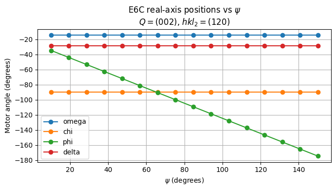
Plot real-axis positions recorded during the scan as a function of $\psi$.
omega, chi, and delta are constant on the chosen solution branch;
phi carries the azimuthal rotation and decreases monotonically.
axis |
data name |
|---|---|
$\varphi$ |
|
$\psi$ |
|
NOTE
ⓘ Extra axes are named with the
_extraslabel inserted in the name.
import matplotlib.pyplot as plt

psi_vals = np.array([d["e6c_hkl_extras_psi"] for d in scan_data])

fig, ax = plt.subplots(figsize=(7, 4))
for motor in ("e6c_hkl_omega", "e6c_hkl_chi", "e6c_hkl_phi", "e6c_hkl_delta"):
    label = motor.removeprefix("e6c_hkl_")
    vals = np.array([d[motor] for d in scan_data])
    ax.plot(psi_vals, vals, marker="o", label=label)

ax.set_xlabel(r"$\psi$ (degrees)")
ax.set_ylabel("Motor angle (degrees)")
ax.set_title(r"E6C real-axis positions vs $\psi$" + "\n" + r"$Q=(002)$, $hkl_2=(120)$")
ax.legend()
ax.grid(True)
plt.tight_layout()
plt.show()