E4CV : 4-circle diffractometer example#
The IUCr provides a schematic of the 4-circle diffractometer (in horizontal geometry typical of a laboratory instrument).
At X-ray synchrotrons, the vertical geometry is more common due to the polarization of the X-rays.
Note: This example is available as a Jupyter notebook from the hklpy source code website: bluesky/hklpy
Setup the E4CV diffractometer in hklpy#
In hkl E4CV geometry (https://people.debian.org/~picca/hkl/hkl.html#org7ef08ba):
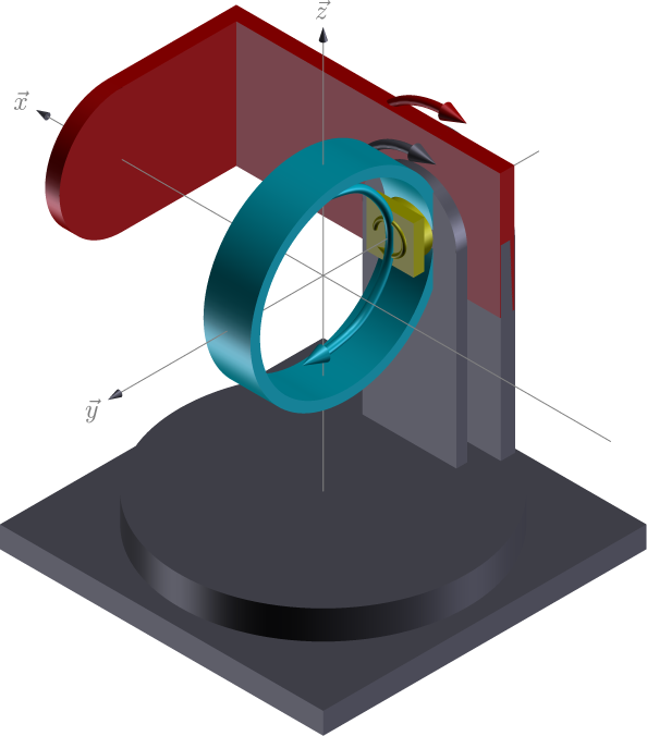
xrays incident on the \(\vec{x}\) direction (1, 0, 0)
axis |
moves |
rotation axis |
vector |
|---|---|---|---|
omega |
sample |
\(-\vec{y}\) |
|
chi |
sample |
\(\vec{x}\) |
|
phi |
sample |
\(-\vec{y}\) |
|
tth |
detector |
\(-\vec{y}\) |
|
Define this diffractometer#
Create a Python class that specifies the names of the real-space positioners. We call it FourCircle here but that choice is arbitrary. Pick any valid Python name not already in use. The convention is to start Python class names with a capital letter and use CamelCase to mark word starts.
The argument to the FourCircle() class tells which hklpy base class will be used. This sets the geometry. (The class we show here could be replaced entirely with hkl.geometries.SimulatedE4CV but we choose to show here the complete steps to produce that class.) The hklpy documentation provides a complete list of diffractometer geometries.
In hklpy, the reciprocal-space axes are known as pseudo positioners while the real-space axes are known as real positioners. For the real positioners, it is possible to use different names than the canonical names used internally by the hkl library. That is not covered here.
Note: The keyword argument kind="hinted" is an indication that this signal may be plotted.
This FourCircle() class example uses simulated motors. See the drop-down for an example how to use EPICS motors.
FourCircle() class using EPICS motors
from hkl import E4CV
from ophyd import EpicsMotor, PseudoSingle
from ophyd import Component as Cpt

class FourCircle(E4CV):
    """
    Our 4-circle.  Eulerian.  Vertical scattering orientation.
    """
    # the reciprocal axes are called "pseudo" in hklpy
    h = Cpt(PseudoSingle, "", kind="hinted")
    k = Cpt(PseudoSingle, "", kind="hinted")
    l = Cpt(PseudoSingle, "", kind="hinted")

    # the motor axes are called "real" in hklpy
    omega = Cpt(EpicsMotor, "pv_prefix:m41", kind="hinted")
    chi = Cpt(EpicsMotor, "pv_prefix:m22", kind="hinted")
    phi = Cpt(EpicsMotor, "pv_prefix:m35", kind="hinted")
    tth = Cpt(EpicsMotor, "pv_prefix:m7", kind="hinted")
[1]:
from hkl import E4CV, SimMixin
from ophyd import SoftPositioner
from ophyd import Component as Cpt

class FourCircle(SimMixin, E4CV):
    """
    Our 4-circle.  Eulerian, vertical scattering orientation.
    """
    # the reciprocal axes are defined by SimMixin

    omega = Cpt(SoftPositioner, kind="hinted", init_pos=0)
    chi = Cpt(SoftPositioner, kind="hinted", init_pos=0)
    phi = Cpt(SoftPositioner, kind="hinted", init_pos=0)
    tth = Cpt(SoftPositioner, kind="hinted", init_pos=0)
Create the Python diffractometer object (fourc) using the FourCircle() class. By convention, the name keyword is the same as the object name.
[2]:
fourc = FourCircle("", name="fourc")
Add a sample with a crystal structure#
[3]:
from hkl import Lattice
from hkl import SI_LATTICE_PARAMETER

# add the sample to the calculation engine
a0 = SI_LATTICE_PARAMETER
fourc.calc.new_sample(
    "silicon",
    lattice=Lattice(a=a0, b=a0, c=a0, alpha=90, beta=90, gamma=90)
    )
[3]:
HklSample(name='silicon', lattice=LatticeTuple(a=5.431020511, b=5.431020511, c=5.431020511, alpha=90.0, beta=90.0, gamma=90.0), ux=Parameter(name='None (internally: ux)', limits=(min=-180.0, max=180.0), value=0.0, fit=True, inverted=False, units='Degree'), uy=Parameter(name='None (internally: uy)', limits=(min=-180.0, max=180.0), value=0.0, fit=True, inverted=False, units='Degree'), uz=Parameter(name='None (internally: uz)', limits=(min=-180.0, max=180.0), value=0.0, fit=True, inverted=False, units='Degree'), U=array([[1., 0., 0.],
       [0., 1., 0.],
       [0., 0., 1.]]), UB=array([[ 1.15690694e+00, -7.08401189e-17, -7.08401189e-17],
       [ 0.00000000e+00,  1.15690694e+00, -7.08401189e-17],
       [ 0.00000000e+00,  0.00000000e+00,  1.15690694e+00]]), reflections=[])
Setup the UB orientation matrix using hklpy#
Define the crystal’s orientation on the diffractometer using the 2-reflection method described by Busing & Levy, Acta Cryst 22 (1967) 457.
Set the same X-ray wavelength for both reflections, by setting the diffractometer energy#
[4]:
from hkl import A_KEV
fourc.energy.put(A_KEV / 1.54)  # (8.0509 keV)
Specify the first reflection and identify its Miller indices: (hkl)#
[5]:
r1 = fourc.calc.sample.add_reflection(
    4, 0, 0,
    position=fourc.calc.Position(
        tth=69.0966,
        omega=-145.451,
        chi=0,
        phi=0,
    )
)
Specify the second reflection#
[6]:
r2 = fourc.calc.sample.add_reflection(
    0, 4, 0,
    position=fourc.calc.Position(
        tth=69.0966,
        omega=-145.451,
        chi=90,
        phi=0,
    )
)
Compute the UB orientation matrix#
The add_reflection() method uses the current wavelength at the time it is called. (To add reflections at different wavelengths, change the wavelength before calling add_reflection() each time.) The compute_UB() method returns the computed UB matrix. Ignore it here.
[7]:
fourc.calc.sample.compute_UB(r1, r2)
[7]:
array([[-1.41342846e-05, -1.41342846e-05, -1.15690694e+00],
       [ 0.00000000e+00, -1.15690694e+00,  1.41342846e-05],
       [-1.15690694e+00,  1.72682934e-10,  1.41342846e-05]])
Report what we have setup#
[8]:
fourc.pa()
===================== ===========================================================================
term                  value
===================== ===========================================================================
diffractometer        fourc
geometry              E4CV
class                 FourCircle
energy (keV)          8.05092
wavelength (angstrom) 1.54000
calc engine           hkl
mode                  bissector
positions             ===== =======
                      name  value
                      ===== =======
                      omega 0.00000
                      chi   0.00000
                      phi   0.00000
                      tth   0.00000
                      ===== =======
constraints           ===== ========= ========== ===== ====
                      axis  low_limit high_limit value fit
                      ===== ========= ========== ===== ====
                      omega -180.0    180.0      0.0   True
                      chi   -180.0    180.0      0.0   True
                      phi   -180.0    180.0      0.0   True
                      tth   -180.0    180.0      0.0   True
                      ===== ========= ========== ===== ====
sample: silicon       ================= =========================================================
                      term              value
                      ================= =========================================================
                      unit cell edges   a=5.431020511, b=5.431020511, c=5.431020511
                      unit cell angles  alpha=90.0, beta=90.0, gamma=90.0
                      ref 1 (hkl)       h=4.0, k=0.0, l=0.0
                      ref 1 positioners omega=-145.45100, chi=0.00000, phi=0.00000, tth=69.09660
                      ref 2 (hkl)       h=0.0, k=4.0, l=0.0
                      ref 2 positioners omega=-145.45100, chi=90.00000, phi=0.00000, tth=69.09660
                      [U]               [[-1.22173048e-05 -1.22173048e-05 -1.00000000e+00]
                                         [ 0.00000000e+00 -1.00000000e+00  1.22173048e-05]
                                         [-1.00000000e+00  1.49262536e-10  1.22173048e-05]]
                      [UB]              [[-1.41342846e-05 -1.41342846e-05 -1.15690694e+00]
                                         [ 0.00000000e+00 -1.15690694e+00  1.41342846e-05]
                                         [-1.15690694e+00  1.72682934e-10  1.41342846e-05]]
                      ================= =========================================================
===================== ===========================================================================
[8]:
<pyRestTable.rest_table.Table at 0x7fb1af7b3450>
Check the orientation matrix#
Perform checks with forward (hkl to angle) and inverse (angle to hkl) computations to verify the diffractometer will move to the same positions where the reflections were identified.
Constrain the motors to limited ranges#
allow for slight roundoff errors
keep
tthin the positive rangekeep
omegain the negative rangekeep
phifixed at zero
First, we apply constraints directly to the calc-level support.
[9]:
fourc.calc["tth"].limits = (-0.001, 180)
fourc.calc["omega"].limits = (-180, 0.001)
fourc.show_constraints()

fourc.phi.move(0)
fourc.engine.mode = "constant_phi"
===== ========= ========== ===== ====
axis  low_limit high_limit value fit
===== ========= ========== ===== ====
omega -180.0    0.001      0.0   True
chi   -180.0    180.0      0.0   True
phi   -180.0    180.0      0.0   True
tth   -0.001    180.0      0.0   True
===== ========= ========== ===== ====
Next, we show how to use additional methods of Diffractometer() that support undo and reset features for applied constraints. The support is based on a stack (a Python list). A set of constraints is added (apply_constraints()) or removed (undo_last_constraints()) from the stack. Or, the stack can be cleared (reset_constraints()).
method |
what happens |
|---|---|
|
Add a set of constraints and use them |
|
Remove the most-recent set of constraints and restore the previous one from the stack. |
|
Set constraints back to initial settings. |
|
Print the current constraints in a table. |
A set of constraints is a Python dictionary that uses the real positioner names (the motors) as the keys. Only those constraints with changes need be added to the dictionary but it is permissable to describe all the real positioners. Each value in the dictionary is a hkl.diffract.Constraint, where the values are specified in this order: low_limit, high_limit, value, fit.
Apply new constraints using the applyConstraints() method. These add to the existing constraints, as shown in the table.
[10]:
from hkl import Constraint
fourc.apply_constraints(
    {
        "tth": Constraint(-0.001, 90, 0, True),
        "chi": Constraint(-90, 90, 0, True),
    }
)
fourc.show_constraints()
===== ========= ========== ===== ====
axis  low_limit high_limit value fit
===== ========= ========== ===== ====
omega -180.0    0.001      0.0   True
chi   -90.0     90.0       0.0   True
phi   -180.0    180.0      0.0   True
tth   -0.001    90.0       0.0   True
===== ========= ========== ===== ====
[10]:
<pyRestTable.rest_table.Table at 0x7fb1af98d450>
Then remove (undo) those new additions.
[11]:
fourc.undo_last_constraints()
fourc.show_constraints()
===== ========= ========== ===== ====
axis  low_limit high_limit value fit
===== ========= ========== ===== ====
omega -180.0    0.001      0.0   True
chi   -180.0    180.0      0.0   True
phi   -180.0    180.0      0.0   True
tth   -0.001    180.0      0.0   True
===== ========= ========== ===== ====
[11]:
<pyRestTable.rest_table.Table at 0x7fb1af7fb090>
(400) reflection test#
Check the
inverse(angles -> (hkl)) computation.Check the
forward((hkl) -> angles) computation.
Check the inverse calculation: (400)#
To calculate the (hkl) corresponding to a given set of motor angles, call fourc.inverse((h, k, l)). Note the second set of parentheses needed by this function.
The values are specified, without names, in the order specified by fourc.calc.physical_axis_names.
[12]:
print("axis names:", fourc.calc.physical_axis_names)
axis names: ['omega', 'chi', 'phi', 'tth']
Now, proceed with the inverse calculation.
[13]:
sol = fourc.inverse((-145.451, 0, 0, 69.0966))
print(f"(4 0 0) ? {sol.h:.2f} {sol.k:.2f} {sol.l:.2f}")
(4 0 0) ? 4.00 0.00 0.00
Check the forward calculation: (400)#
Compute the angles necessary to position the diffractometer for the given reflection.
Note that for the forward computation, more than one set of angles may be used to reach the same crystal reflection. This test will report the default selection. The default selection (which may be changed through methods described in the hkl.calc module) is the first solution.
function |
returns |
|---|---|
|
The default solution |
|
List of all allowed solutions. |
Here we print the default solution (the one returned by calling fourc.forward()).
[14]:
sol = fourc.forward((4, 0, 0))
print(
    "(400) :",
    f"tth={sol.tth:.4f}",
    f"omega={sol.omega:.4f}",
    f"chi={sol.chi:.4f}",
    f"phi={sol.phi:.4f}"
    )
(400) : tth=69.0982 omega=-145.4502 chi=-0.0000 phi=0.0000
(040) reflection test#
Repeat the inverse and forward calculations for the second orientation reflection.
Check the inverse calculation: (040)#
[15]:
sol = fourc.inverse((-145.451, 90, 0, 69.0966))
print(f"(0 4 0) ? {sol.h:.2f} {sol.k:.2f} {sol.l:.2f}")
(0 4 0) ? 0.00 4.00 0.00
Check the forward calculation: (040)#
[16]:
sol = fourc.forward((0, 4, 0))
print(
    "(040) :",
    f"tth={sol.tth:.4f}",
    f"omega={sol.omega:.4f}",
    f"chi={sol.chi:.4f}",
    f"phi={sol.phi:.4f}"
    )
(040) : tth=69.0982 omega=-145.4502 chi=90.0000 phi=0.0000
Scan in reciprocal space using Bluesky#
To scan with Bluesky, we need more setup.
[17]:
%matplotlib inline

from bluesky import RunEngine
from bluesky import SupplementalData
from bluesky.callbacks.best_effort import BestEffortCallback
from bluesky.magics import BlueskyMagics
import bluesky.plans as bp
import bluesky.plan_stubs as bps
import databroker
from IPython import get_ipython
import matplotlib.pyplot as plt

plt.ion()

bec = BestEffortCallback()
db = databroker.temp().v1
sd = SupplementalData()

get_ipython().register_magics(BlueskyMagics)

RE = RunEngine({})
RE.md = {}
RE.preprocessors.append(sd)
RE.subscribe(db.insert)
RE.subscribe(bec)
[17]:
1
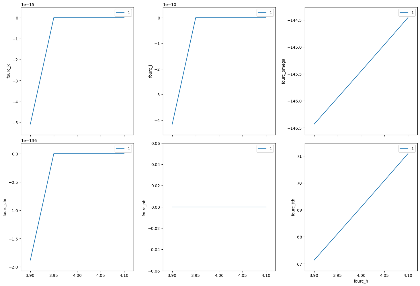
(h00) scan near (400)#
In this example, we have no detector. Still, we add the diffractometer object in the detector list so that the hkl and motor positions will appear as columns in the table.
[18]:
RE(bp.scan([fourc], fourc.h, 3.9, 4.1, 5))
Transient Scan ID: 1     Time: 2023-11-20 21:54:23
Persistent Unique Scan ID: '09df1bc7-c0f4-4602-838a-d951148e9bbc'
New stream: 'primary'
+-----------+------------+------------+------------+------------+-------------+------------+------------+------------+
|   seq_num |       time |    fourc_h |    fourc_k |    fourc_l | fourc_omega |  fourc_chi |  fourc_phi |  fourc_tth |
+-----------+------------+------------+------------+------------+-------------+------------+------------+------------+
|         1 | 21:54:24.1 |      3.900 |     -0.000 |     -0.000 |    -146.431 |     -0.000 |      0.000 |     67.137 |
|         2 | 21:54:24.7 |      3.950 |     -0.000 |     -0.000 |    -145.942 |      0.000 |      0.000 |     68.115 |
|         3 | 21:54:25.3 |      4.000 |     -0.000 |     -0.000 |    -145.450 |     -0.000 |      0.000 |     69.098 |
|         4 | 21:54:25.9 |      4.050 |     -0.000 |      0.000 |    -144.956 |     -0.000 |      0.000 |     70.087 |
|         5 | 21:54:26.5 |      4.100 |     -0.000 |     -0.000 |    -144.458 |     -0.000 |      0.000 |     71.083 |
+-----------+------------+------------+------------+------------+-------------+------------+------------+------------+
generator scan ['09df1bc7'] (scan num: 1)
/home/prjemian/.conda/envs/bluesky_2023_3/lib/python3.11/site-packages/bluesky/callbacks/fitting.py:167: RuntimeWarning: invalid value encountered in scalar divide
  np.sum(input * grids[dir].astype(float), labels, index) / normalizer
[18]:
('09df1bc7-c0f4-4602-838a-d951148e9bbc',)
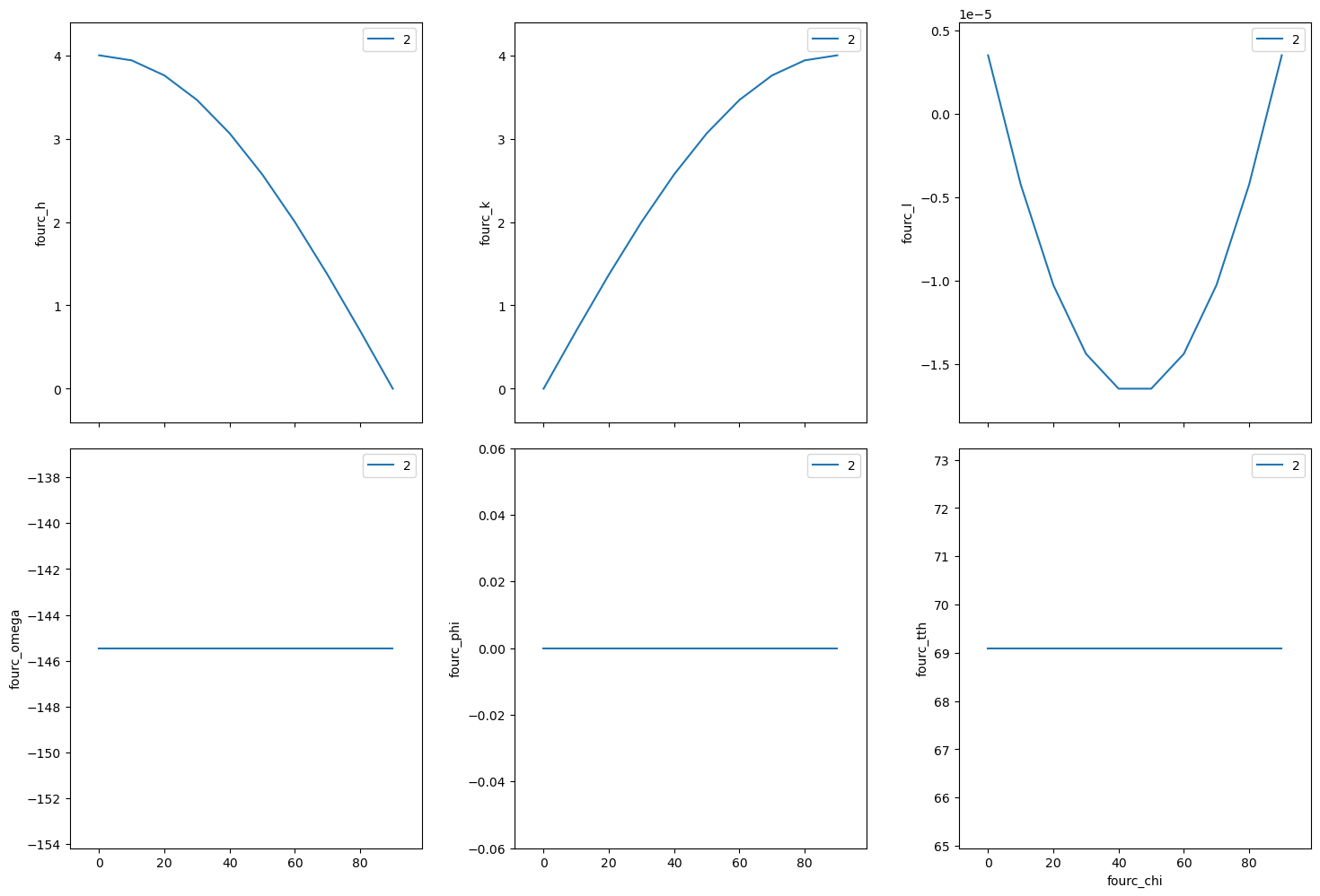
chi scan from (400) to (040)#
If we do this with \(\omega=-145.4500\) and \(2\theta=69.0985\), this will be a scan between the two orientation reflections.
Use %mov (IPython magic command) to move both motors at the same time.
[19]:
print("possible modes:", fourc.calc.engine.modes)
print("chosen mode:", fourc.calc.engine.mode)

# same as orientation reflections
%mov fourc.omega -145.4500 fourc.tth 69.0985

RE(bp.scan([fourc], fourc.chi, 0, 90, 10))
possible modes: ['bissector', 'constant_omega', 'constant_chi', 'constant_phi', 'double_diffraction', 'psi_constant']
chosen mode: constant_phi


Transient Scan ID: 2     Time: 2023-11-20 21:54:28
Persistent Unique Scan ID: '9e38d630-10e7-4d08-8235-631f06794940'
New stream: 'primary'
+-----------+------------+------------+------------+------------+------------+-------------+------------+------------+
|   seq_num |       time |  fourc_chi |    fourc_h |    fourc_k |    fourc_l | fourc_omega |  fourc_phi |  fourc_tth |
+-----------+------------+------------+------------+------------+------------+-------------+------------+------------+
|         1 | 21:54:28.4 |      0.000 |      4.000 |      0.000 |      0.000 |    -145.450 |      0.000 |     69.099 |
|         2 | 21:54:29.0 |     10.000 |      3.939 |      0.695 |     -0.000 |    -145.450 |      0.000 |     69.099 |
|         3 | 21:54:29.6 |     20.000 |      3.759 |      1.368 |     -0.000 |    -145.450 |      0.000 |     69.099 |
|         4 | 21:54:30.1 |     30.000 |      3.464 |      2.000 |     -0.000 |    -145.450 |      0.000 |     69.099 |
|         5 | 21:54:30.7 |     40.000 |      3.064 |      2.571 |     -0.000 |    -145.450 |      0.000 |     69.099 |
|         6 | 21:54:31.3 |     50.000 |      2.571 |      3.064 |     -0.000 |    -145.450 |      0.000 |     69.099 |
|         7 | 21:54:31.9 |     60.000 |      2.000 |      3.464 |     -0.000 |    -145.450 |      0.000 |     69.099 |
|         8 | 21:54:32.5 |     70.000 |      1.368 |      3.759 |     -0.000 |    -145.450 |      0.000 |     69.099 |
|         9 | 21:54:33.1 |     80.000 |      0.695 |      3.939 |     -0.000 |    -145.450 |      0.000 |     69.099 |
|        10 | 21:54:33.6 |     90.000 |      0.000 |      4.000 |      0.000 |    -145.450 |      0.000 |     69.099 |
+-----------+------------+------------+------------+------------+------------+-------------+------------+------------+
generator scan ['9e38d630'] (scan num: 2)
[19]:
('9e38d630-10e7-4d08-8235-631f06794940',)
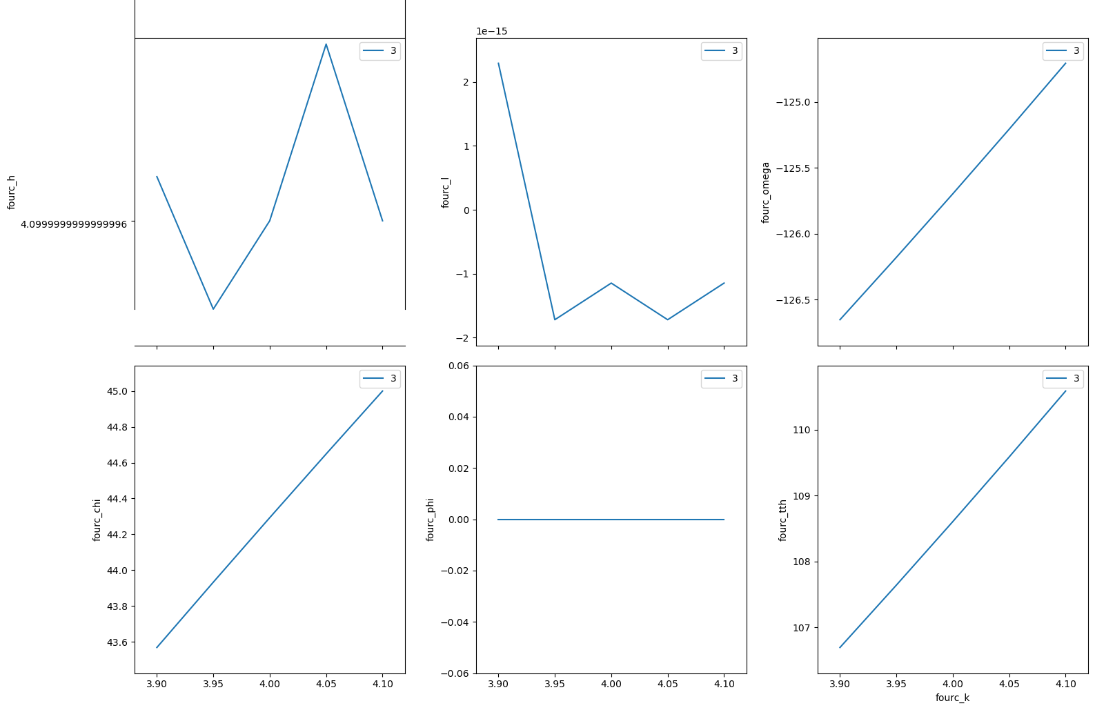
(0k0) scan near (040)#
[20]:
RE(bp.scan([fourc], fourc.k, 3.9, 4.1, 5))
Transient Scan ID: 3     Time: 2023-11-20 21:54:35
Persistent Unique Scan ID: '855bb64b-0056-4bbb-8c88-ccdd4248a8f8'
New stream: 'primary'
+-----------+------------+------------+------------+------------+-------------+------------+------------+------------+
|   seq_num |       time |    fourc_k |    fourc_h |    fourc_l | fourc_omega |  fourc_chi |  fourc_phi |  fourc_tth |
+-----------+------------+------------+------------+------------+-------------+------------+------------+------------+
|         1 | 21:54:35.4 |      3.900 |      4.100 |      0.000 |    -126.652 |     43.568 |      0.000 |    106.695 |
|         2 | 21:54:36.0 |      3.950 |      4.100 |     -0.000 |    -126.179 |     43.933 |      0.000 |    107.641 |
|         3 | 21:54:36.5 |      4.000 |      4.100 |     -0.000 |    -125.697 |     44.293 |      0.000 |    108.604 |
|         4 | 21:54:37.1 |      4.050 |      4.100 |     -0.000 |    -125.206 |     44.648 |      0.000 |    109.585 |
|         5 | 21:54:37.7 |      4.100 |      4.100 |     -0.000 |    -124.707 |     45.000 |      0.000 |    110.585 |
+-----------+------------+------------+------------+------------+-------------+------------+------------+------------+
generator scan ['855bb64b'] (scan num: 3)
[20]:
('855bb64b-0056-4bbb-8c88-ccdd4248a8f8',)
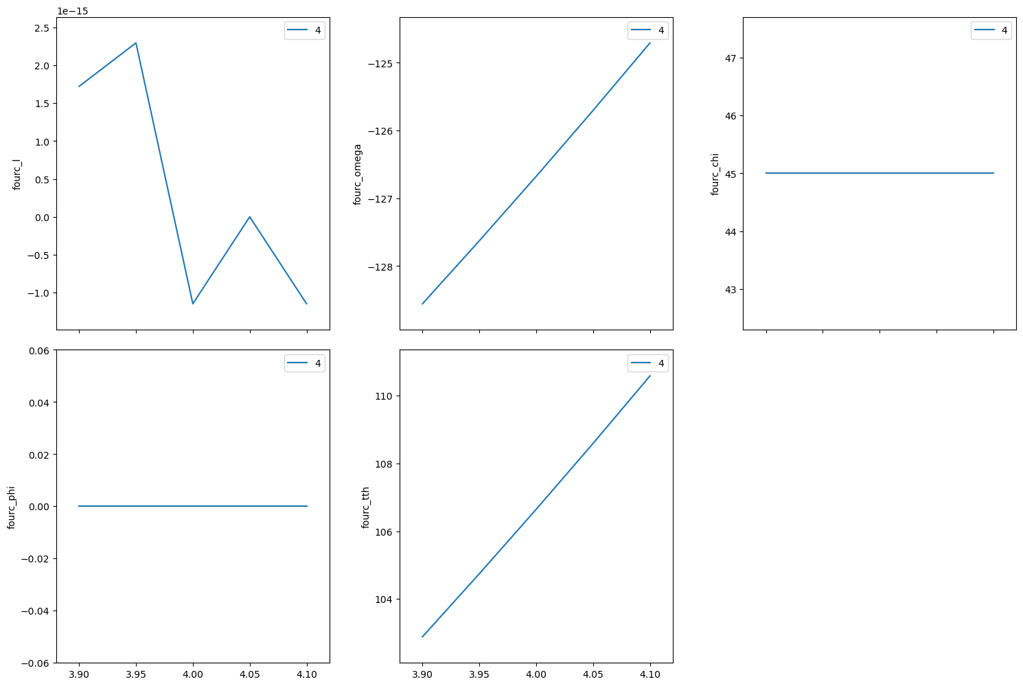
(hk0) scan near (440)#
[21]:
RE(bp.scan([fourc], fourc.h, 3.9, 4.1, fourc.k, 3.9, 4.1, 5))
Transient Scan ID: 4     Time: 2023-11-20 21:54:39
Persistent Unique Scan ID: 'df5e8dae-b0ed-48a5-9e12-ca1fbdb8fdf4'
New stream: 'primary'
+-----------+------------+------------+------------+------------+-------------+------------+------------+------------+
|   seq_num |       time |    fourc_h |    fourc_k |    fourc_l | fourc_omega |  fourc_chi |  fourc_phi |  fourc_tth |
+-----------+------------+------------+------------+------------+-------------+------------+------------+------------+
|         1 | 21:54:39.4 |      3.900 |      3.900 |      0.000 |    -128.558 |     45.000 |      0.000 |    102.882 |
|         2 | 21:54:39.8 |      3.950 |      3.950 |      0.000 |    -127.627 |     45.000 |      0.000 |    104.744 |
|         3 | 21:54:40.3 |      4.000 |      4.000 |     -0.000 |    -126.676 |     45.000 |      0.000 |    106.647 |
|         4 | 21:54:40.7 |      4.050 |      4.050 |      0.000 |    -125.703 |     45.000 |      0.000 |    108.592 |
|         5 | 21:54:41.1 |      4.100 |      4.100 |     -0.000 |    -124.707 |     45.000 |      0.000 |    110.585 |
+-----------+------------+------------+------------+------------+-------------+------------+------------+------------+
generator scan ['df5e8dae'] (scan num: 4)
[21]:
('df5e8dae-b0ed-48a5-9e12-ca1fbdb8fdf4',)
Move to the (440) reflection.
[22]:
fourc.move((4,4,0))
print(f"{fourc.position = }")
fourc.position = FourCirclePseudoPos(h=4.0, k=4.000000000000001, l=5.735944501465638e-16)
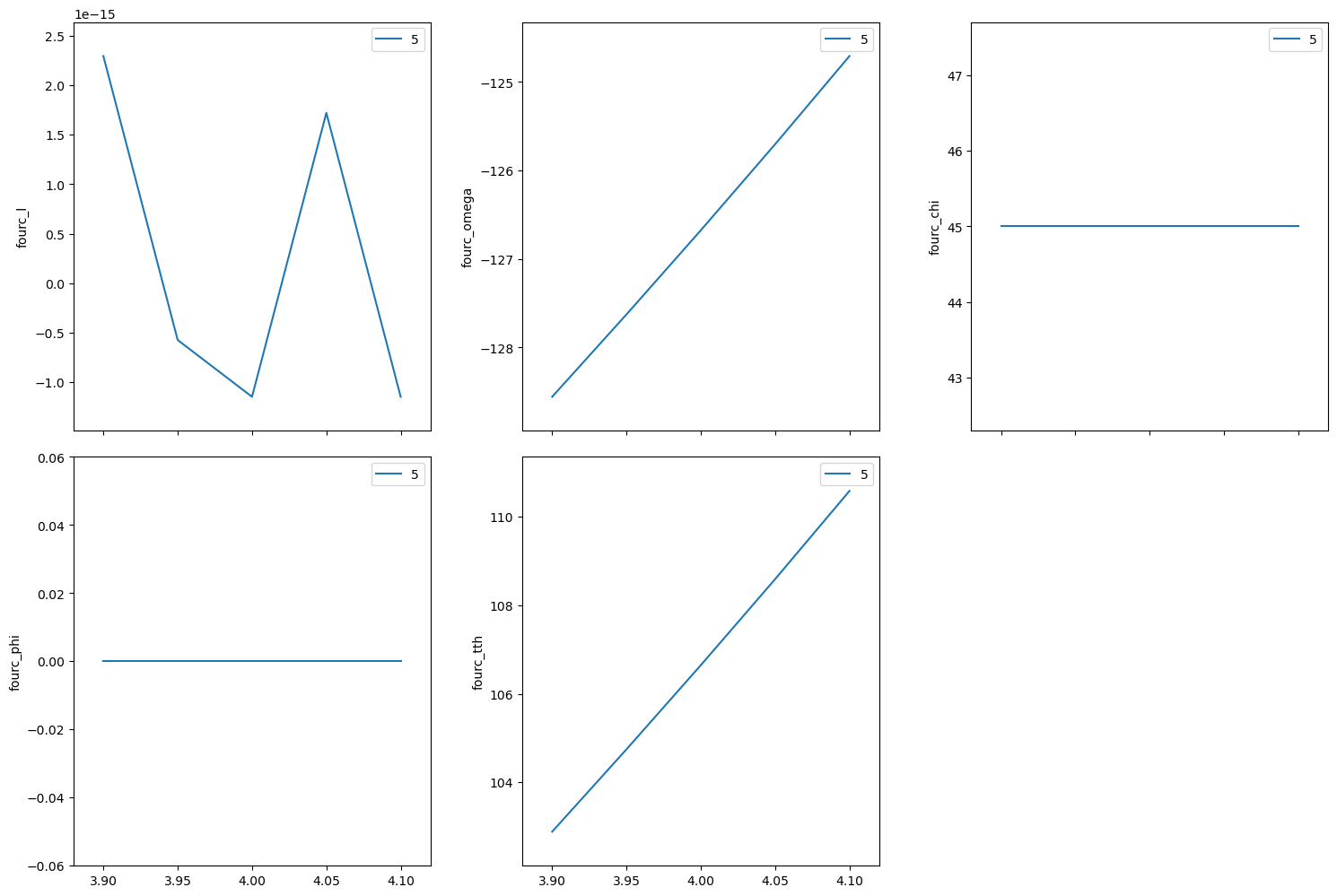
Repeat the same scan about the (440) but use relative positions.
[23]:
RE(bp.rel_scan([fourc], fourc.h, -0.1, 0.1, fourc.k, -0.1, 0.1, 5))
Transient Scan ID: 5     Time: 2023-11-20 21:54:42
Persistent Unique Scan ID: '9fd485f8-1438-46d1-98b3-e499283579bc'
New stream: 'primary'
+-----------+------------+------------+------------+------------+-------------+------------+------------+------------+
|   seq_num |       time |    fourc_h |    fourc_k |    fourc_l | fourc_omega |  fourc_chi |  fourc_phi |  fourc_tth |
+-----------+------------+------------+------------+------------+-------------+------------+------------+------------+
|         1 | 21:54:42.6 |      3.900 |      3.900 |      0.000 |    -128.558 |     45.000 |      0.000 |    102.882 |
|         2 | 21:54:43.0 |      3.950 |      3.950 |     -0.000 |    -127.627 |     45.000 |      0.000 |    104.744 |
|         3 | 21:54:43.4 |      4.000 |      4.000 |     -0.000 |    -126.676 |     45.000 |      0.000 |    106.647 |
|         4 | 21:54:43.8 |      4.050 |      4.050 |      0.000 |    -125.703 |     45.000 |      0.000 |    108.592 |
|         5 | 21:54:44.3 |      4.100 |      4.100 |     -0.000 |    -124.707 |     45.000 |      0.000 |    110.585 |
+-----------+------------+------------+------------+------------+-------------+------------+------------+------------+
generator rel_scan ['9fd485f8'] (scan num: 5)
[23]:
('9fd485f8-1438-46d1-98b3-e499283579bc',)