Plans#

A plan is bluesky’s concept of an experimental procedure. A plan may be any iterable object (list, tuple, custom iterable class, …) but most commonly it is implemented as a Python generator. For a more technical discussion we refer you Message Protocol.

A variety of pre-assembled plans are provided. Like sandwiches on a deli menu, you can use our pre-assembled plans or assemble your own from the same ingredients, catalogued under the heading Stub Plans below.

Note

In the examples that follow, we will assume that you have a RunEngine instance named RE. This may have already been configured for you if you are a user at a facility that runs bluesky. See this section of the tutorial to sort out if you already have a RunEngine and to quickly make one if needed.

Pre-assembled Plans#

Below this summary table, we break the down the plans by category and show examples with figures.

Summary#

Notice that the names in the left column are links to detailed API documentation.

`count`	Take one or more readings from detectors.
`scan`	Scan over one multi-motor trajectory.
`rel_scan`	Scan over one multi-motor trajectory relative to current position.
`list_scan`	Scan over one or more variables in steps simultaneously (inner product).
`rel_list_scan`	Scan over one variable in steps relative to current position.
`list_grid_scan`	Scan over a mesh; each motor is on an independent trajectory.
`rel_list_grid_scan`	Scan over a mesh; each motor is on an independent trajectory.
`log_scan`	Scan over one variable in log-spaced steps.
`rel_log_scan`	Scan over one variable in log-spaced steps relative to current position.
`grid_scan`	Scan over a mesh; each motor is on an independent trajectory.
`rel_grid_scan`	Scan over a mesh relative to current position.
`scan_nd`	Scan over an arbitrary N-dimensional trajectory.
`spiral`	Spiral scan, centered around (x_start, y_start)
`spiral_fermat`	Absolute fermat spiral scan, centered around (x_start, y_start)
`spiral_square`	Absolute square spiral scan, centered around (x_center, y_center)
`rel_spiral`	Relative spiral scan
`rel_spiral_fermat`	Relative fermat spiral scan
`rel_spiral_square`	Relative square spiral scan, centered around current (x, y) position.
`adaptive_scan`	Scan over one variable with adaptively tuned step size.
`rel_adaptive_scan`	Relative scan over one variable with adaptively tuned step size.
`tune_centroid`	plan: tune a motor to the centroid of signal(motor)
`tweak`	Move and motor and read a detector with an interactive prompt.
`ramp_plan`	Take data while ramping one or more positioners.
`fly`	Perform a fly scan with one or more 'flyers'.

Time series (“count”)#

Examples:

from ophyd.sim import det
from bluesky.plans import count

# a single reading of the detector 'det'
RE(count([det]))

# five consecutive readings
RE(count([det], num=5))

# five sequential readings separated by a 1-second delay
RE(count([det], num=5, delay=1))

# a variable delay
RE(count([det], num=5, delay=[1, 2, 3, 4]))

# Take readings forever, until interrupted (e.g., with Ctrl+C)
RE(count([det], num=None))

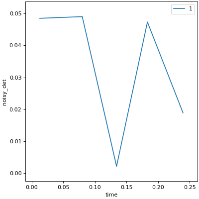
# We'll use the 'noisy_det' example detector for a more interesting plot.
from ophyd.sim import noisy_det

RE(count([noisy_det], num=5))

Note

Why doesn’t count() have an exposure_time parameter?

Modern CCD detectors typically parametrize exposure time with multiple parameters (acquire time, acquire period, num exposures, …) as do scalers (preset time, auto count time). There is no one “exposure time” that can be applied to all detectors.

Additionally, when using multiple detectors as in count([det1, det2])), the user would need to provide a separate exposure time for each detector in the general case, which would grow wordy.

One option is to set the time-related parameter(s) as a separate step.

For interactive use:

# Just an example. Your detector might have different names or numbers of
# exposure-related parameters---which is the point.
det.exposure_time.set(3)
det.acquire_period.set(3.5)

From a plan:

# Just an example. Your detector might have different names or numbers of
# exposure-related parameters---which is the point.
 yield from bluesky.plan_stubs.mv(
     det.exposure_time, 3,
     det.acquire_period, 3.5)

Another is to write a custom plan that wraps count() and sets the exposure time. This plan can encode the details that bluesky in general can’t know.

def count_with_time(detectors, num, delay, exposure_time, *, md=None):
    # Assume all detectors have one exposure time component called
    # 'exposure_time' that fully specifies its exposure.
    for detector in detectors:
        yield from bluesky.plan_stubs.mv(detector.exposure_time, exposure_time)
    yield from bluesky.plans.count(detectors, num, delay, md=md)

count

Take one or more readings from detectors.

Scans over one dimension#

The “dimension” might be a physical motor position, a temperature, or a pseudo-axis. It’s all the same to the plans. Examples:

from ophyd.sim import det, motor
from bluesky.plans import scan, rel_scan, list_scan

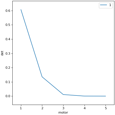
# scan a motor from 1 to 5, taking 5 equally-spaced readings of 'det'
RE(scan([det], motor, 1, 5, 5))

# scan a motor from 1 to 5 *relative to its current position*
RE(rel_scan([det], motor, 1, 5, 5))

# scan a motor through a list of user-specified positions
RE(list_scan([det], motor, [1, 1, 2, 3, 5, 8]))

RE(scan([det], motor, 1, 5, 5))

Note

Why don’t scans have a delay parameter?

You may have noticed that count() has a delay parameter but none of the scans do. This is intentional.

The common reason for wanting a delay in a scan is to allow a motor to settle or a temperature controller to reach equilibrium. It is better to configure this on the respective devices, so that scans will always add the appropriate delay for the particular device being scanned.

motor.settle_time = 1
temperature_controller.settle_time = 10

For many cases, this is more convenient and more robust than typing a delay parameter in every invocation of the scan. You only have to set it once, and it applies thereafter.

This is why bluesky leaves delay out of the scans, to guide users toward an approach that will likely be a better fit than the one that might occur to them first. For situations where a delay parameter really is the right tool for the job, it is of course always possible to add a delay parameter yourself by writing a custom plan. Here is one approach, using a per_step hook.

import bluesky.plans
import bluesky.plan_stubs

def scan_with_delay(*args, delay=0, **kwargs):
    "Accepts all the normal 'scan' parameters, plus an optional delay."

    def one_nd_step_with_delay(detectors, step, pos_cache):
        "This is a copy of bluesky.plan_stubs.one_nd_step with a sleep added."
        motors = step.keys()
        yield from bluesky.plan_stubs.move_per_step(step, pos_cache)
        yield from bluesky.plan_stubs.sleep(delay)
        yield from bluesky.plan_stubs.trigger_and_read(list(detectors) + list(motors))

    kwargs.setdefault('per_step', one_nd_step_with_delay)
    yield from bluesky.plans.scan(*args, **kwargs)

`scan`	Scan over one multi-motor trajectory.
`rel_scan`	Scan over one multi-motor trajectory relative to current position.
`list_scan`	Scan over one or more variables in steps simultaneously (inner product).
`rel_list_scan`	Scan over one variable in steps relative to current position.
`log_scan`	Scan over one variable in log-spaced steps.
`rel_log_scan`	Scan over one variable in log-spaced steps relative to current position.

Multi-dimensional scans#

See Scan Multiple Motors Together in the tutorial for an introduction to the common cases of moving multiple motors in coordination (i.e. moving X and Y along a diagonal) or in a grid. The key examples are reproduced here. Again, see the section linked for further explanation.

from ophyd.sim import det, motor1, motor2, motor3
from bluesky.plans import scan, grid_scan, list_scan, list_grid_scan

RE(scan(dets,
        motor1, -1.5, 1.5,  # scan motor1 from -1.5 to 1.5
        motor2, -0.1, 0.1,  # ...while scanning motor2 from -0.1 to 0.1
        11))  # ...both in 11 steps

# Scan motor1 and motor2 jointly through a 5-point trajectory.
RE(list_scan(dets, motor1, [1, 1, 3, 5, 8], motor2, [25, 16, 9, 4, 1]))

# Scan a 3 x 5 x 2 grid.
RE(grid_scan([det],
             motor1, -1.5, 1.5, 3,  # no snake parameter for first motor
             motor2, -0.1, 0.1, 5, False))
             motor3, -200, 200, 5, False))

# Scan a grid with abitrary spacings given as specific positions.
RE(list_grid_scan([det],
                  motor1, [1, 1, 2, 3, 5],
                  motor2, [25, 16, 9]))

All of these plans are built on a more general-purpose plan, scan_nd(), which we can use for more specialized cases.

Some jargon: we speak of scan()-like joint movement as an “inner product” of trajectories and grid_scan()-like movement as an “outer product” of trajectories. The general case, moving some motors together in an “inner product” against another motor (or motors) in an “outer product,” can be addressed using a cycler. Notice what happens when we add or multiply cycler objects.

In [1]: from cycler import cycler

In [2]: from ophyd.sim import motor1, motor2, motor3

In [3]: traj1 = cycler(motor1, [1, 2, 3])

In [4]: traj2 = cycler(motor2, [10, 20, 30])

In [5]: list(traj1)  # a trajectory for motor1
Out[5]: 
[{SynAxis(prefix='', name='motor1', read_attrs=['readback', 'setpoint'], configuration_attrs=['velocity', 'acceleration']): 1},
 {SynAxis(prefix='', name='motor1', read_attrs=['readback', 'setpoint'], configuration_attrs=['velocity', 'acceleration']): 2},
 {SynAxis(prefix='', name='motor1', read_attrs=['readback', 'setpoint'], configuration_attrs=['velocity', 'acceleration']): 3}]

In [6]: list(traj1 + traj2)  # an "inner product" trajectory
Out[6]: 
[{SynAxis(prefix='', name='motor1', read_attrs=['readback', 'setpoint'], configuration_attrs=['velocity', 'acceleration']): 1,
  SynAxis(prefix='', name='motor2', read_attrs=['readback', 'setpoint'], configuration_attrs=['velocity', 'acceleration']): 10},
 {SynAxis(prefix='', name='motor1', read_attrs=['readback', 'setpoint'], configuration_attrs=['velocity', 'acceleration']): 2,
  SynAxis(prefix='', name='motor2', read_attrs=['readback', 'setpoint'], configuration_attrs=['velocity', 'acceleration']): 20},
 {SynAxis(prefix='', name='motor1', read_attrs=['readback', 'setpoint'], configuration_attrs=['velocity', 'acceleration']): 3,
  SynAxis(prefix='', name='motor2', read_attrs=['readback', 'setpoint'], configuration_attrs=['velocity', 'acceleration']): 30}]

In [7]: list(traj1 * traj2)  # an "outer product" trajectory
Out[7]: 
[{SynAxis(prefix='', name='motor1', read_attrs=['readback', 'setpoint'], configuration_attrs=['velocity', 'acceleration']): 1,
  SynAxis(prefix='', name='motor2', read_attrs=['readback', 'setpoint'], configuration_attrs=['velocity', 'acceleration']): 10},
 {SynAxis(prefix='', name='motor1', read_attrs=['readback', 'setpoint'], configuration_attrs=['velocity', 'acceleration']): 1,
  SynAxis(prefix='', name='motor2', read_attrs=['readback', 'setpoint'], configuration_attrs=['velocity', 'acceleration']): 20},
 {SynAxis(prefix='', name='motor1', read_attrs=['readback', 'setpoint'], configuration_attrs=['velocity', 'acceleration']): 1,
  SynAxis(prefix='', name='motor2', read_attrs=['readback', 'setpoint'], configuration_attrs=['velocity', 'acceleration']): 30},
 {SynAxis(prefix='', name='motor1', read_attrs=['readback', 'setpoint'], configuration_attrs=['velocity', 'acceleration']): 2,
  SynAxis(prefix='', name='motor2', read_attrs=['readback', 'setpoint'], configuration_attrs=['velocity', 'acceleration']): 10},
 {SynAxis(prefix='', name='motor1', read_attrs=['readback', 'setpoint'], configuration_attrs=['velocity', 'acceleration']): 2,
  SynAxis(prefix='', name='motor2', read_attrs=['readback', 'setpoint'], configuration_attrs=['velocity', 'acceleration']): 20},
 {SynAxis(prefix='', name='motor1', read_attrs=['readback', 'setpoint'], configuration_attrs=['velocity', 'acceleration']): 2,
  SynAxis(prefix='', name='motor2', read_attrs=['readback', 'setpoint'], configuration_attrs=['velocity', 'acceleration']): 30},
 {SynAxis(prefix='', name='motor1', read_attrs=['readback', 'setpoint'], configuration_attrs=['velocity', 'acceleration']): 3,
  SynAxis(prefix='', name='motor2', read_attrs=['readback', 'setpoint'], configuration_attrs=['velocity', 'acceleration']): 10},
 {SynAxis(prefix='', name='motor1', read_attrs=['readback', 'setpoint'], configuration_attrs=['velocity', 'acceleration']): 3,
  SynAxis(prefix='', name='motor2', read_attrs=['readback', 'setpoint'], configuration_attrs=['velocity', 'acceleration']): 20},
 {SynAxis(prefix='', name='motor1', read_attrs=['readback', 'setpoint'], configuration_attrs=['velocity', 'acceleration']): 3,
  SynAxis(prefix='', name='motor2', read_attrs=['readback', 'setpoint'], configuration_attrs=['velocity', 'acceleration']): 30}]

We have reproduced inner product and outer product. The real power comes in when we combine them, like so. Here, motor1 and motor2 together in a mesh against motor3.

In [8]: traj3 = cycler(motor3, [100, 200, 300])

In [9]: list((traj1 + traj2) * traj3)
Out[9]: 
[{SynAxis(prefix='', name='motor1', read_attrs=['readback', 'setpoint'], configuration_attrs=['velocity', 'acceleration']): 1,
  SynAxis(prefix='', name='motor2', read_attrs=['readback', 'setpoint'], configuration_attrs=['velocity', 'acceleration']): 10,
  SynAxis(prefix='', name='motor3', read_attrs=['readback', 'setpoint'], configuration_attrs=['velocity', 'acceleration']): 100},
 {SynAxis(prefix='', name='motor1', read_attrs=['readback', 'setpoint'], configuration_attrs=['velocity', 'acceleration']): 1,
  SynAxis(prefix='', name='motor2', read_attrs=['readback', 'setpoint'], configuration_attrs=['velocity', 'acceleration']): 10,
  SynAxis(prefix='', name='motor3', read_attrs=['readback', 'setpoint'], configuration_attrs=['velocity', 'acceleration']): 200},
 {SynAxis(prefix='', name='motor1', read_attrs=['readback', 'setpoint'], configuration_attrs=['velocity', 'acceleration']): 1,
  SynAxis(prefix='', name='motor2', read_attrs=['readback', 'setpoint'], configuration_attrs=['velocity', 'acceleration']): 10,
  SynAxis(prefix='', name='motor3', read_attrs=['readback', 'setpoint'], configuration_attrs=['velocity', 'acceleration']): 300},
 {SynAxis(prefix='', name='motor1', read_attrs=['readback', 'setpoint'], configuration_attrs=['velocity', 'acceleration']): 2,
  SynAxis(prefix='', name='motor2', read_attrs=['readback', 'setpoint'], configuration_attrs=['velocity', 'acceleration']): 20,
  SynAxis(prefix='', name='motor3', read_attrs=['readback', 'setpoint'], configuration_attrs=['velocity', 'acceleration']): 100},
 {SynAxis(prefix='', name='motor1', read_attrs=['readback', 'setpoint'], configuration_attrs=['velocity', 'acceleration']): 2,
  SynAxis(prefix='', name='motor2', read_attrs=['readback', 'setpoint'], configuration_attrs=['velocity', 'acceleration']): 20,
  SynAxis(prefix='', name='motor3', read_attrs=['readback', 'setpoint'], configuration_attrs=['velocity', 'acceleration']): 200},
 {SynAxis(prefix='', name='motor1', read_attrs=['readback', 'setpoint'], configuration_attrs=['velocity', 'acceleration']): 2,
  SynAxis(prefix='', name='motor2', read_attrs=['readback', 'setpoint'], configuration_attrs=['velocity', 'acceleration']): 20,
  SynAxis(prefix='', name='motor3', read_attrs=['readback', 'setpoint'], configuration_attrs=['velocity', 'acceleration']): 300},
 {SynAxis(prefix='', name='motor1', read_attrs=['readback', 'setpoint'], configuration_attrs=['velocity', 'acceleration']): 3,
  SynAxis(prefix='', name='motor2', read_attrs=['readback', 'setpoint'], configuration_attrs=['velocity', 'acceleration']): 30,
  SynAxis(prefix='', name='motor3', read_attrs=['readback', 'setpoint'], configuration_attrs=['velocity', 'acceleration']): 100},
 {SynAxis(prefix='', name='motor1', read_attrs=['readback', 'setpoint'], configuration_attrs=['velocity', 'acceleration']): 3,
  SynAxis(prefix='', name='motor2', read_attrs=['readback', 'setpoint'], configuration_attrs=['velocity', 'acceleration']): 30,
  SynAxis(prefix='', name='motor3', read_attrs=['readback', 'setpoint'], configuration_attrs=['velocity', 'acceleration']): 200},
 {SynAxis(prefix='', name='motor1', read_attrs=['readback', 'setpoint'], configuration_attrs=['velocity', 'acceleration']): 3,
  SynAxis(prefix='', name='motor2', read_attrs=['readback', 'setpoint'], configuration_attrs=['velocity', 'acceleration']): 30,
  SynAxis(prefix='', name='motor3', read_attrs=['readback', 'setpoint'], configuration_attrs=['velocity', 'acceleration']): 300}]

For more on cycler, we refer you to the cycler documentation. To build a plan incorporating these trajectories, use our general N-dimensional scan plan, scan_nd().

RE(scan_nd([det], (traj1 + traj2) * traj3))

`scan`	Scan over one multi-motor trajectory.
`rel_scan`	Scan over one multi-motor trajectory relative to current position.
`grid_scan`	Scan over a mesh; each motor is on an independent trajectory.
`rel_grid_scan`	Scan over a mesh relative to current position.
`list_scan`	Scan over one or more variables in steps simultaneously (inner product).
`rel_list_scan`	Scan over one variable in steps relative to current position.
`list_grid_scan`	Scan over a mesh; each motor is on an independent trajectory.
`rel_list_grid_scan`	Scan over a mesh; each motor is on an independent trajectory.
`scan_nd`	Scan over an arbitrary N-dimensional trajectory.

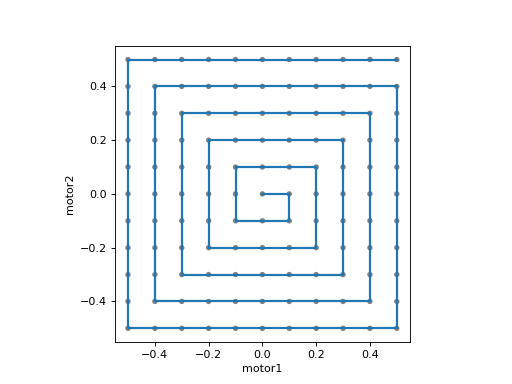
Spiral trajectories#

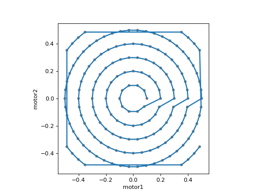
We provide two-dimensional scans that trace out spiral trajectories.

A simple spiral:

from bluesky.simulators import plot_raster_path
from ophyd.sim import motor1, motor2, det
from bluesky.plans import spiral

plan = spiral([det], motor1, motor2, x_start=0.0, y_start=0.0, x_range=1.,
              y_range=1.0, dr=0.1, nth=10)
plot_raster_path(plan, 'motor1', 'motor2', probe_size=.01)

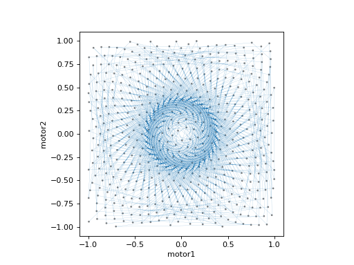
A fermat spiral:

from bluesky.simulators import plot_raster_path
from ophyd.sim import motor1, motor2, det
from bluesky.plans import spiral_fermat

plan = spiral_fermat([det], motor1, motor2, x_start=0.0, y_start=0.0,
                     x_range=2.0, y_range=2.0, dr=0.1, factor=2.0, tilt=0.0)
plot_raster_path(plan, 'motor1', 'motor2', probe_size=.01, lw=0.1)

A square spiral:

from bluesky.simulators import plot_raster_path
from ophyd.sim import motor1, motor2, det
from bluesky.plans import spiral_square

plan = spiral_square([det], motor1, motor2, x_center=0.0, y_center=0.0,
                     x_range=1.0, y_range=1.0, x_num=11, y_num=11)
plot_raster_path(plan, 'motor1', 'motor2', probe_size=.01)

`spiral`	Spiral scan, centered around (x_start, y_start)
`spiral_fermat`	Absolute fermat spiral scan, centered around (x_start, y_start)
`spiral_square`	Absolute square spiral scan, centered around (x_center, y_center)
`rel_spiral`	Relative spiral scan
`rel_spiral_fermat`	Relative fermat spiral scan
`rel_spiral_square`	Relative square spiral scan, centered around current (x, y) position.

Adaptive scans#

These are one-dimension scans with an adaptive step size tuned to move quickly over flat regions can concentrate readings in areas of high variation by computing the local slope aiming for a target delta y between consecutive points.

This is a basic example of the power of adaptive plan logic.

from bluesky.plans import adaptive_scan
from ophyd.sim import motor, det

RE(adaptive_scan([det], 'det', motor,
                 start=-15,
                 stop=10,
                 min_step=0.01,
                 max_step=5,
                 target_delta=.05,
                 backstep=True))

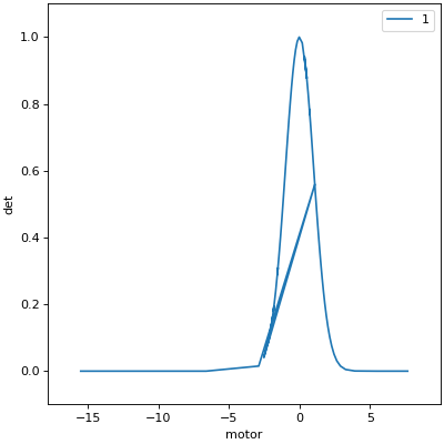
From left to right, the scan lengthens its stride through the flat region. At first, it steps past the peak. The large jump causes it to double back and then sample more densely through the peak. As the peak flattens, it lengthens its stride again.

`adaptive_scan`	Scan over one variable with adaptively tuned step size.
`rel_adaptive_scan`	Relative scan over one variable with adaptively tuned step size.

Misc.#

`tweak`	Move and motor and read a detector with an interactive prompt.
`fly`	Perform a fly scan with one or more 'flyers'.

Stub Plans#

These are the aforementioned “ingredients” for remixing, the pieces from which the pre-assembled plans above were made. See Write Custom Plans in the tutorial for a practical introduction to these components.

Plans for interacting with hardware:

`abs_set`	Set a value.
`rel_set`	Set a value relative to current value.
`mv`	Move one or more devices to a setpoint.
`mvr`	Move one or more devices to a relative setpoint.
`trigger`	Trigger and acquisition.
`read`	Take a reading and add it to the current bundle of readings.
`rd`	Reads a single-value non-triggered object
`stage`	'Stage' a device (i.e., prepare it for use, 'arm' it).
`unstage`	'Unstage' a device (i.e., put it in standby, 'disarm' it).
`configure`	Change Device configuration and emit an updated Event Descriptor document.
`stop`	Stop a device.

Plans for asynchronous acquisition:

`monitor`	Asynchronously monitor for new values and emit Event documents.
`unmonitor`	Stop monitoring.
`kickoff`	Kickoff one fly-scanning device.
`complete`	Tell a flyable, 'stop collecting, whenever you are ready'.
`collect`	Collect data cached by one or more fly-scanning devices and emit documents.

Plans that control the RunEngine:

`open_run`	Mark the beginning of a new 'run'.
`close_run`	Mark the end of the current 'run'.
`create`	Bundle future readings into a new Event document.
`save`	Close a bundle of readings and emit a completed Event document.
`drop`	Drop a bundle of readings without emitting a completed Event document.
`pause`	Pause and wait for the user to resume.
`deferred_pause`	Pause at the next checkpoint.
`checkpoint`	If interrupted, rewind to this point.
`clear_checkpoint`	Designate that it is not safe to resume.
`sleep`	Tell the RunEngine to sleep, while asynchronously doing other processing.
`input_plan`	Prompt the user for text input.
`subscribe`	Subscribe the stream of emitted documents.
`unsubscribe`	Remove a subscription.
`install_suspender`	Install a suspender during a plan.
`remove_suspender`	Remove a suspender during a plan.
`wait`	Wait for all statuses in a group to report being finished.
`wait_for`	Low-level: wait for a list of `asyncio.Future` objects to set (complete).
`null`	Yield a no-op Message.

Combinations of the above that are often convenient:

`trigger_and_read`(devices[, name])	Trigger and read a list of detectors and bundle readings into one Event.
`one_1d_step`(detectors, motor, step[, ...])	Inner loop of a 1D step scan
`one_nd_step`(detectors, step, pos_cache[, ...])	Inner loop of an N-dimensional step scan
`one_shot`(detectors[, take_reading])	Inner loop of a count.
`move_per_step`(step, pos_cache)	Inner loop of an N-dimensional step scan without any readings

Special utilities:

`repeat`(plan[, num, delay])	Repeat a plan num times with delay and checkpoint between each repeat.
`repeater`(n, gen_func, args, *kwargs)	Generate n chained copies of the messages from gen_func
`caching_repeater`(n, plan)	Generate n chained copies of the messages in a plan.
`broadcast_msg`(command, objs, args, *kwargs)	Generate many copies of a message, applying it to a list of devices.

Plan Preprocessors#

Supplemental Data#

Plan preprocessors modify a plans contents on the fly. One common use of a preprocessor is to take “baseline” readings of a group of devices at the beginning and end of each run. It is convenient to apply this to all plans executed by a RunEngine using the SupplementalData.

class bluesky.preprocessors.SupplementalData(*, baseline=None, monitors=None, flyers=None)[source]#

A configurable preprocessor for supplemental measurements

This is a plan preprocessor. It inserts messages into plans to:

take “baseline” readings at the beginning and end of each run for the devices listed in its baseline atrribute
monitor signals in its monitors attribute for asynchronous updates during each run.
kick off “flyable” devices listed in its flyers attribute at the beginning of each run and collect their data at the end

Internally, it uses the plan preprocessors:

Parameters:

baselinelist: Devices to be read at the beginning and end of each run
monitorslist: Signals (not multi-signal Devices) to be monitored during each run, generating readings asynchronously
flyerslist: “Flyable” Devices to be kicked off before each run and collected at the end of each run

Examples

Create an instance of SupplementalData and apply it to a RunEngine.

>>> sd = SupplementalData(baseline=[some_motor, some_detector]),
...                       monitors=[some_signal],
...                       flyers=[some_flyer])
>>> RE = RunEngine({})
>>> RE.preprocessors.append(sd)

Now all plans executed by RE will be modified to add baseline readings (before and after each run), monitors (during each run), and flyers (kicked off before each run and collected afterward).

Inspect or update the lists of devices interactively.

>>> sd.baseline
[some_motor, some_detector]

>>> sd.baseline.remove(some_motor)

>>> sd.baseline
[some_detector]

>>> sd.baseline.append(another_detector)

>>> sd.baseline
[some_detector, another_detector]

Each attribute (baseline, monitors, flyers) is an ordinary Python list, support all the standard list methods, such as:

>>> sd.baseline.clear()

The arguments to SupplementalData are optional. All the lists will empty by default. As shown above, they can be populated interactively.

>>> sd = SupplementalData()
>>> RE = RunEngine({})
>>> RE.preprocessors.append(sd)
>>> sd.baseline.append(some_detector)

We have installed a “preprocessor” on the RunEngine. A preprocessor modifies plans, supplementing or altering their instructions in some way. From now on, every time we type RE(some_plan()), the RunEngine will silently change some_plan() to sd(some_plan()), where sd may insert some extra instructions. Envision the instructions flow from some_plan to sd and finally to RE. The sd preprocessors has the opportunity to inspect he instructions as they go by and modify them as it sees fit before they get processed by the RunEngine.

Preprocessor Wrappers and Decorators#

Preprocessors can make arbirary modifcations to a plan, and can get quite devious. For example, the relative_set_wrapper() rewrites all positions to be relative to the initial position.

def rel_scan(detectors, motor, start, stop, num):
    absolute = scan(detectors, motor, start, stop, num)
    relative = relative_set_wrapper(absolute, [motor])
    yield from relative

This is a subtle but remarkably powerful feature.

Wrappers like relative_set_wrapper() operate on a generator instance, like scan(...). There are corresponding decorator functions like relative_set_decorator that operate on a generator function itself, like scan().

# Using a decorator to modify a generator function
def rel_scan(detectors, motor, start, stop, num):

    @relative_set_decorator([motor])  # unfamiliar syntax? -- see box below
    def inner_relative_scan():
        yield from scan(detectors, motor, start, stop, num)

    yield from inner_relative_scan()

Incidentally, the name inner_relative_scan is just an internal variable, so why did we choose such a verbose name? Why not just name it f? That would work, of course, but using a descriptive name can make debugging easier. When navigating gnarly, deeply nested tracebacks, it helps if internal variables have clear names.

Note

The decorator syntax — the @ — is a succinct way of passing a function to another function.

This:

@g
def f(...):
    pass

f(...)

is equivalent to

g(f)(...)

Built-in Preprocessors#

Each of the following functions named <something>_wrapper operates on a generator instance. The corresponding functions named <something_decorator> operate on a generator function.

`baseline_decorator`	Preprocessor that records a baseline of all devices after open_run
`baseline_wrapper`	Preprocessor that records a baseline of all devices after open_run
`contingency_wrapper`	try...except...else...finally helper
`finalize_decorator`	try...finally helper
`finalize_wrapper`	try...finally helper
`fly_during_decorator`	Kickoff and collect "flyer" (asynchronously collect) objects during runs.
`fly_during_wrapper`	Kickoff and collect "flyer" (asynchronously collect) objects during runs.
`inject_md_decorator`	Inject additional metadata into a run.
`inject_md_wrapper`	Inject additional metadata into a run.
`lazily_stage_decorator`	This is a preprocessor that inserts 'stage' messages and appends 'unstage'.
`lazily_stage_wrapper`	This is a preprocessor that inserts 'stage' messages and appends 'unstage'.
`monitor_during_decorator`	Monitor (asynchronously read) devices during runs.
`monitor_during_wrapper`	Monitor (asynchronously read) devices during runs.
`relative_set_decorator`	Interpret 'set' messages on devices as relative to initial position.
`relative_set_wrapper`	Interpret 'set' messages on devices as relative to initial position.
`reset_positions_decorator`	Return movable devices to their initial positions at the end.
`reset_positions_wrapper`	Return movable devices to their initial positions at the end.
`run_decorator`	Enclose in 'open_run' and 'close_run' messages.
`run_wrapper`	Enclose in 'open_run' and 'close_run' messages.
`stage_decorator`	'Stage' devices (i.e., prepare them for use, 'arm' them) and then unstage.
`stage_wrapper`	'Stage' devices (i.e., prepare them for use, 'arm' them) and then unstage.
`subs_decorator`	Subscribe callbacks to the document stream; finally, unsubscribe.
`subs_wrapper`	Subscribe callbacks to the document stream; finally, unsubscribe.
`suspend_decorator`	Install suspenders to the RunEngine, and remove them at the end.
`suspend_wrapper`	Install suspenders to the RunEngine, and remove them at the end.

Custom Preprocessors#

The preprocessors are implemented using msg_mutator() (for altering messages in place) and plan_mutator() (for inserting messages into the plan or removing messages).

It’s easiest to learn this by example, studying the implementations of the built-in processors (catalogued above) in the the source of the plans module.

Customize Step Scans with `per_step`#

The one-dimensional and multi-dimensional plans are composed (1) setup, (2) a loop over a plan to perform at each position, (3) cleanup.

We provide a hook for customizing step (2). This enables you to write a variation of an existing plan without starting from scratch.

For one-dimensional plans, the default inner loop is:

from bluesky.plan_stubs import checkpoint, abs_set, trigger_and_read

def one_1d_step(detectors, motor, step):
    """
    Inner loop of a 1D step scan

    This is the default function for ``per_step`` param in 1D plans.
    """
    yield from checkpoint()
    yield from abs_set(motor, step, wait=True)
    return (yield from trigger_and_read(list(detectors) + [motor]))

Some user-defined function, custom_step, with the same signature can be used in its place:

scan([det], motor, 1, 5, 5, per_step=custom_step)

For convenience, this could be wrapped into the definition of a new plan:

def custom_scan(detectors, motor, start, stop, step, *, md=None):
    yield from scan([det], motor, start, stop, step, md=md
                    per_step=custom_step)

For multi-dimensional plans, the default inner loop is:

from bluesky.utils import short_uid
from bluesky.plan_stubs import checkpoint, abs_set, wait, trigger_and_read

def one_nd_step(detectors, step, pos_cache):
    """
    Inner loop of an N-dimensional step scan

    This is the default function for ``per_step`` param in ND plans.

    Parameters
    ----------
    detectors : iterable
        devices to read
    step : dict
        mapping motors to positions in this step
    pos_cache : dict
        mapping motors to their last-set positions
    """
    def move():
        yield from checkpoint()
        grp = short_uid('set')
        for motor, pos in step.items():
            if pos == pos_cache[motor]:
                # This step does not move this motor.
                continue
            yield from abs_set(motor, pos, group=grp)
            pos_cache[motor] = pos
        yield from wait(group=grp)

    motors = step.keys()
    yield from move()
    yield from trigger_and_read(list(detectors) + list(motors))

Likewise, a custom function with the same signature may be passed into the per_step argument of any of the multi-dimensional plans.

Asynchronous Plans: “Fly Scans” and “Monitoring”#

See the section on Asynchronous Acquisition for some context on these terms and, near the end of the section, some example plans.

Plan Utilities#

These are useful utilities for defining custom plans and plan preprocessors.

`pchain`	Like itertools.chain but using yield from
`msg_mutator`	A simple preprocessor that mutates or deletes single messages in a plan.
`plan_mutator`	Alter the contents of a plan on the fly by changing or inserting messages.
`single_gen`	Turn a single message into a plan
`make_decorator`	Turn a generator instance wrapper into a generator function decorator.

Plans#

Pre-assembled Plans#

Summary#

Time series (“count”)#

Scans over one dimension#

Multi-dimensional scans#

Spiral trajectories#

Adaptive scans#

Misc.#

Stub Plans#

Plan Preprocessors#

Supplemental Data#

Preprocessor Wrappers and Decorators#

Built-in Preprocessors#

Custom Preprocessors#

Customize Step Scans with per_step#

Asynchronous Plans: “Fly Scans” and “Monitoring”#

Plan Utilities#

Customize Step Scans with `per_step`#